
The introduction of three-dimensional (3D) electromagnetic (EM) Simulation launched a revolution in microwave design by allowing engineers to design, analyze and refine 3D microwave components on their computers. For the first time, designers could visualize the electromagnetic fields in their device, understand the device’s electrical behavior to an unprecedented degree and build virtual products that work as predicted when manufactured. As EM simulation technology evolves, it continues to transform and define RF and microwave design.
The trend in RF and microwave design is towards the accurate prediction of system-level performance and behavior. Engineers simulate larger and more sophisticated design problems in support of that goal. In antenna design, for example, phased-array antenna system designers are not only simulating the antenna element(s), but also the supporting feed network and active circuits behind the array. Other antenna system designers are focusing on the environment in which the antenna operates—the performance of an antenna beneath a radome, for example, or the interaction of a mobile handset with the body of an automobile. In short, the size and complexity of problems being addressed by electromagnetic simulations have grown enormously.
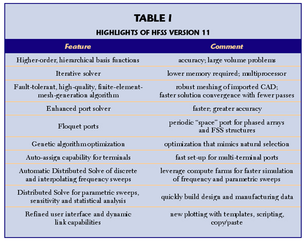
To enable larger, system-level design, developers of the widely used EM simulator, HFSS, have focused on product features and new technology that deliver even greater accuracy, capacity and performance than before. HFSS Version 11 includes new higher-order hierarchical basis functions combined with an iterative solver that provides accurate fields using fewer mesh elements. This provides more efficient solutions for large multi-wavelength structures. A new fault-tolerant, high-quality finite-element-meshing algorithm allows HFSS to simulate very complex models two to five times faster using half the memory compared to previous versions. Continued user interface refinement and data linking enables co-design of complex electronic systems. This article discusses some of the new technology in HFSS version 11 (see Table 1) and highlights examples illustrating the new level of speed, accuracy and memory efficiency.
Phased-array Antenna on Aircraft

The following example demonstrates technology specific to HFSS that supports antenna system design. Figure 1 shows an overview of an antenna system and platform installation. The system consists of a four-element Vivaldi antenna array mounted within the radome of a fixed-wing aircraft. The array is fed by active transmit/receive circuits that use traditional microstrip circuit technologies and monolithic microwave integrated circuit (MMIC) low-noise and power amplifiers.
For over a decade, microwave circuits have been designed with distributed transmission-line techniques. Advanced electromagnetic simulators have been used to complement the analysis by providing more detailed physical extraction. However, these traditional approaches have had limitations. Antennas and their operating environments are often 3D and therefore do not have circuit models. New technologies that couple electromagnetic and circuit simulation are extending these traditional techniques to complex 3D structures like the tapered slot (Vivaldi) antenna shown in Figure 1. In addition, these technologies support various system-level analyses—the feed network and antenna array system or the antenna and radome system, for example. In particular, new technologies called Dynamic Link, Pushed Excitations and Data Link enable complex antenna system simulation.
Dynamic Link is a technology that provides bi-directional connection between circuit and electromagnetic simulators. Fully parameterized electromagnetic models are linked to circuits with parameters such as dimensions and material properties passed to the electromagnetic simulator and S-parameter results passed back. Multi-dimensional interpolation between solved dimensions in the electromagnetic models provides the speed of circuit simulation with the accuracy of full-wave electromagnetics.
Pushed Excitations is a technology that closes the loop between circuits and electromagnetics. Circuit simulation produces the voltages and currents on all nodes and all branches of the circuit, respectively. Those voltages and currents can be used as the excitation to the electromagnetic model so that engineers can visualize fields and compute secondary radiation patterns. This can be done without re-solving the finite element problem because Pushed Excitations simply scale the HFSS result by applying the excitations at HFSS ports.
Data Link couples multiple HFSS simulation projects by linking tangential fields on the outer surface of one HFSS project to another. This linkage between projects allows engineers to efficiently simulate very large and complex geometries.

Optimizing the Tapered Slot Profile
Figure 2 illustrates how the Dynamic Link and Pushed Excitations were used to optimize the taper profile of a single Vivaldi antenna element. The project starts by using HFSS’s unique capability to create frequency dependent circuit models of arbitrary geometries. By combining these models with a distributed parametric sweep of selected variables and dynamically linking to the circuit, “tunable” distributed circuit models can be realized. Once the dynamically linked, slot-line components are cascaded in circuit, the simulation achieves the accuracy of 3D electromagnetics with the speed of circuit simulation. Through real-time tuning of the circuit with subsequent feedback from HFSS, the optimal taper profile was identified. With the optimal taper profile, circuit excitations are pushed to the HFSS model so that the resulting far field patterns, shown at the bottom of Figure 2, may be visualized.
Testing the Array and Feed Network
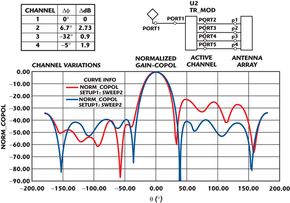
Using the optimized Vivaldi element, a 1 x 4 linear array is assembled and extracted in HFSS. To simulate system performance, the antenna array is dynamically linked to the active circuit network. In addition to the base excitations required for normal incidence, one test employed phase and amplitude variations to simulate the effects of manufacturing tolerances. Pushed excitations were used to visualize and predict the antenna system’s performance under the various test conditions. Figure 3 shows the “variation” test case (red) versus the ideal normal incidence case (blue) where no variation in amplitude or phasing was employed. As shown in the figure, the result of the manufacturing tolerances was an increase in side lobe levels.
The final validation of the system is obtained by installing the antenna array and feed network on an unmanned, fixed wing platform. Here, all three technologies were used to simulate the phased array with the active circuits adjusted to achieve a 22° beam scan. The resulting currents and voltages were pushed to the terminals of the antenna to determine the radiated fields, which included the effect of the feed circuitry. Finally, the Data Link technology is used to compute the fields of this antenna when placed beneath a radome on an aircraft, as shown in Figure 4. As can be seen in the figure, the calculated fields produced inside and outside the radome are consistent with a 22° beam scan.
Advanced Technology in HFSS

The previous phased array example was solved using HFSS Version 11 and leveraged new solver technology to allow the large simulations. Some of these technologies will now be discussed, including higher-order hierarchical basis functions, iterative solver, and the finite-element-meshing algorithm that allows HFSS to simulate bigger and more complex geometries.
Hierarchical Basis
The finite-element method as implemented in HFSS works by dividing a 3D problem space into tetrahedral-shaped elements. The electric field in each of these tetrahedrons can be interpolated from the values associated with the edges, faces and volume of the tetrahedron. HFSS stores the components of the field that are tangential to the six edges and four faces of the tetrahedron. In addition, HFSS can store the vector components of the field within the volume of the tetrahedron. The field inside each tetrahedron is interpolated from these values.
Various interpolation schemes, or basis functions, can be used to interpolate field values from the nodal values shown in Figure 5. Zero-order tangential elements have six unknowns per tetrahedron. A zero-order basis function assumes that the tangential component of the field is constant along each edge. First-order tangential elements have 20 unknowns per tetrahedron. Twelve of these unknowns arise from assuming that the tangential component of the first-order tangential element basis function is linear along each edge. The remaining eight unknowns are added to ensure completeness of the polynomial and are normal to the edges but tangential to the faces. Second-order tangential element basis functions have 45 unknowns including 18 unknowns associated with the edges, 24 unknowns associated with the faces and three unknowns associated with the volume.
HFSS by default uses first-order elements as these have proved to be the most efficient with general problems. Users of previous versions of HFSS may be familiar with an option within the solution setup panels that allowed them to select “low order” as the solution basis. This feature was useful especially for signal integrity problems such as connectors and printed-circuit escape routing where geometric detail in the model forces a dense finite-element mesh. In these cases, the mesh is denser than required for accurate field prediction; hence, using a low-order (zero) element reduces the total number of unknowns and speeds the solution while maintaining accuracy. With Version 11, there is now the additional option of selecting a second-order element. Second-order elements are useful for geometries containing large homogeneous regions that can be represented by large tetrahedrons using higher-order interpolation.
Iterative Solver
Working hand-in-hand with the hierarchical basis is a new iterative solver. The finite-element formulation produces a matrix equation that must be solved to find the unknown electric field values within the elements. This matrix is sparse because of the local interaction between tetrahedrons. The most memory efficient method for solving a sparse matrix equation is to use an iterative solver (as compared to the more traditional direct-matrix solver). The iterative solver has the advantage of lower memory requirements and faster solutions as long as the process is conditioned properly. HFSS Version 11 uses solutions from lower-order elements to precondition the iterative solver for higher-order elements. Indeed, it is this unique coupling between the hierarchical bases and the matrix solver that makes the iterative procedure practical, reliable and fast.
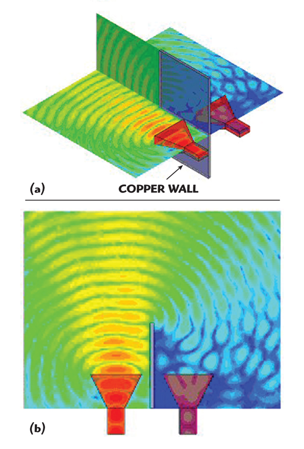
The memory savings benefit of the new matrix solver is made evident by the example demonstrated in Figure 6. Here, two pyramidal horn antennas in the presence of a conducting wall simulates co-site coupling. The geometry is a large 447-cubic-wavelength volume of a homogenous vacuum medium. The simulation was performed using a direct solver and again with Version 11 using the iterative solver. Both solvers converged in three passes; however, the iterative solver required 3.2 times less RAM and was 6.4 times faster than the direct solver.

A further experiment was performed to examine growth of the memory requirements as the number of unknowns is increased. The convergence criterion delta-S was set extremely small to force the number of unknowns to grow to the limits of the memory capacity of the computer. The graph in Figure 7 shows the memory usage of the direct and iterative solvers versus the number of tetrahedrons for each pass. The graph may be interpreted in two different ways. First, for a fixed number of tetrahedrons, the iterative solver uses roughly four times less RAM. In fact, HFSS memory usage is approaching a theoretical minimum because memory usage grows linearly, that is, it doubles with a doubling of the number of unknowns. Alternatively, a second interpretation is that HFSS can solve larger and more complex problems with a fixed amount of computer RAM (6 GB, for example).
Meshing Engine
Version 11 has a new meshing engine that has significant impact on the solution process, speed and memory usage. Many applications require importation of geometries from other computer aided design (CAD) programs. The fault-tolerant meshing engine automatically detects and repairs structural problems with these geometries and optionally allows the user to remove unnecessary details such as chamfers, bends and drill holes.

The new engine creates a higher-quality mesh with well-formed tetrahedrons. The higher-quality mesh combined with further improvements in mesh refinement has resulted in faster convergence for most simulations. HFSS Version 11 often converges with fewer adaptive passes and hence requires less RAM and CPU time. The example of a Vivaldi antenna in Figure 8 illustrates this new performance. The older version required 13 adaptive passes, 2.67 GB RAM and just over 20 minutes to solve. Version 11 only required nine passes, 770 MB RAM and only three minutes to solve. That’s a 6.7 times faster simulation and 2.7 times lower memory requirement.
Conclusion
The need for engineers to solve larger and more complex geometries efficiently is of growing concern. HFSS Version 11 has new features and technologies that provide an engineering solution to address this concern. The combination of a new hierarchical basis, iterative solver and advanced meshing engine push the frontier of electromagnetic simulation. Linking circuits and electromagnetics with features like Dynamic Link, Pushed Excitations and Data Link allows engineers to design and validate entire end-to-end systems before undertaking prototype production.
References
1. T.Y. Yun, C. Wang, P. Zepeda, C.T. Rodenbeck, M.R. Coutant, M. Li and K. Chang, “A 10–21 GHz, Low-cost, Multi-frequency and Full-duplex Phased Array Antenna System,” IEEE Trans. Antennas and Propagation, May 2002, Vol. 50, pp. 641–650.
2. C. Chang, C. Rodenbeck, K. Chang and M. Coutant, “A Four-channel Full-duplex T/R Module for Multi-frequency Phased Array Applications,” Microwave Journal On-line, April 2005.
Ansoft Corp.
Pittsburgh, PA
(412) 261-3200
www.ansoft.com