
The function of a power amplifier (PA) in a radio communications system is to boost a signal to a power level suitable for transmission. In modern RF power amplifier applications, there are two conflicting design requirements: the need for linearity to preserve the fidelity of the signal and the demand for efficiency of the PA.
All RF power amplifiers distort the signals that pass through them. Distortion is defined as the change in the signal shape that occurs when that signal is passed through a nonlinear system. This results in an increase in the number of frequency components present in the output signal when compared to the input signal.
High frequency power amplifiers operate most efficiently at saturation in the nonlinear range of their behavior. In modern communication systems, the signals are amplitude and phase modulated to achieve better spectral efficiency: using the smallest bandwidth to transmit a given amount of information.1 Such signals exhibit a large peak-to-average power ratio (PAR), meaning that the average power of the signal that is to be amplified by the PA can be many times smaller than the peaks of the signal. The PA must be able to handle the peaks, which means that the PA is usually operating well below its peak efficiency point.
Attempts to balance the nonlinearities in saturation against the improved efficiency lead to interesting circuit techniques that often achieve improved efficiency as a result of the control of the harmonic content of the amplified signal, and not simply its elimination as in traditional designs.
A modulated carrier that has amplitude variations will exhibit a spread of the transmitted spectrum (spectral regrowth) as a result of nonlinearities in the amplifier. These new spectral components (distortion) are generated by the nonlinearities of the circuit and degrade the spectral efficiency of the system. Given a known stimulus and a representation of the nonlinear system, these nonlinearities can be derived to explain how they arise.
Nonlinear Analysis of Power Amplifiers
The typical input for a power amplifier in a telecommunications application is usually sinusoidal in nature and contains both amplitude and phase modulation characteristics, which represent the baseband information signal.2 The signal has the following structure
x(t) = A(t)cos[ω ct+θ(t)] (1)
where
A(t) = amplitude modulation (AM) on the input signal
θ(t) = phase modulation (PM) on the signal
Representing the system as a low order polynomial, y(t) = f(x(t)), gives
y L(t) = α1 x(t–τ1) (2)
for linear response when the input signal is small, and a nonlinear response of
yNL(t) = α1 x(t–τ1)
+ α2 x(t–τ2)2 + α3 x(t–τ3)3 +… (3)
The response of the system (linear and nonlinear) to Equation 1 is
yL(t) = α1A(t–τ1) cos[ω ct+θ(t–τ1)–φ1],
φ1 = ω cτ1 (4)
yNL(t) =
α1A(t–τ1) cos[ω ct+θ(t–τ1)–φ1]
+α2A(t–τ2)2 cos[ω ct+θ(t–τ2)–φ2]2
+α3A(t–τ3)3 cos[ω ct+θ(t–τ3)–φ3]3,
φ1 + ω cτ1, φ2 = ω cτ2, φ3 = ω cτ3 (5)
where the expression is truncated to the third degree, ω c represents the carrier frequency and the τi are constant. Using trigonometric identifiers Equation 5 may be rewritten as 

The τi in Equations 2–6 are a result of memory effects.
Memory Effects
RFPA memory effects can be classified as long term or short term. Long-term memory effects, which will not be addressed in this article, are the result of thermal transients, supply variability and electron traps. Short-term electrical memory effects are caused by transistor time delays that are modeled by energy storage elements such as capacitances or inductances.3
With memory, the response of the circuit or system becomes dependent on prior values of the input and the time response of the system is no longer instantaneous. Taking a linear time-invariant capacitor, for example, the voltage across the capacitor at time t is

assuming that there was no initial charge when the capacitor was manufactured.4 If a charge is placed on the capacitor and the voltage is given at t = t0, then Equation 7 becomes

Equation 7 demonstrates that the capacitor voltage, unlike the voltage across a linear resistor, is dependent on the entire past history of the current through the capacitor. Equation 8 shows that knowledge of the entire past history of the capacitor voltage is not required if the voltage is known at some initial time, t0. Equations 7 and 8 can be applied to inductors in a similar fashion.
The resulting effect of these elements is a frequency dependent gain and phase shift of the output signal compared to the input signal. Electrical memory effects add poles and zeros to the response of the linear system causing changes in gain and phase across frequency.
In the nonlinear representation of a system the impact of memory lends greater complexity to the analysis. In PAs in particular, memory effects contribute not only to amplitude distortion (AM-AM) but to phase distortion as well (AM-PM). This will be demonstrated in the analysis in the following section.
Distortion Analysis
The two-tone test is widely used for analysis of communication system components. This test effectively varies the envelope of the input signal through its complete range, testing the amplifier over its entire transfer characteristic3 with the application of a sinusoidal signal to the RF carrier. The two-tone test can reveal both phase and amplitude distortions present in an amplifier. The following evaluation of distortion products will neglect phase modulation for the purpose of simplicity, but the procedure is the same. In the case of a PA, the two-tone input signal stimulating the device is in the form
x(t) = A1cos(ω1t) + A2cos(ω2t) (9)
Rewriting the expressions for the linear and nonlinear responses to a two-tone to include a time delay for systems with memory
yL(t) = α1(A1cos(ω1t–ω1τ)
+ A2cos(ω2t–ω2τ)) (10)
and
yNL(t) = α1(A1cos(ω1t–ω1τ1)
+ A2cos(ω2t–ω2τ1))
+α2(A1cos(ω1t–ω1τ2)
+ A2cos(ω2t–ω2τ2))2
+ α3(A1cos(ω1t–ω1τ3)
+ A2cos(ω2t–ω2τ3))3 =
α1 (A1cos(ω1t–φ11) +A2cos(ω2t–φ21))
+ α2 (A1cos(ω1t–φ12)
+ A2cos(ω2t–φ22))2
+ α3 (A1cos(ω1t–φ13)
v+ A2cos(ω2t–φ23))3,
φ11 = ω1τ1, φ21 = ω2τ1, … φij = ωiτj
(11)
The φij terms in Equation 11 represent the phase shift associated with each polynomial term and are considered constant in this analysis. Equation 11 can then be expanded to
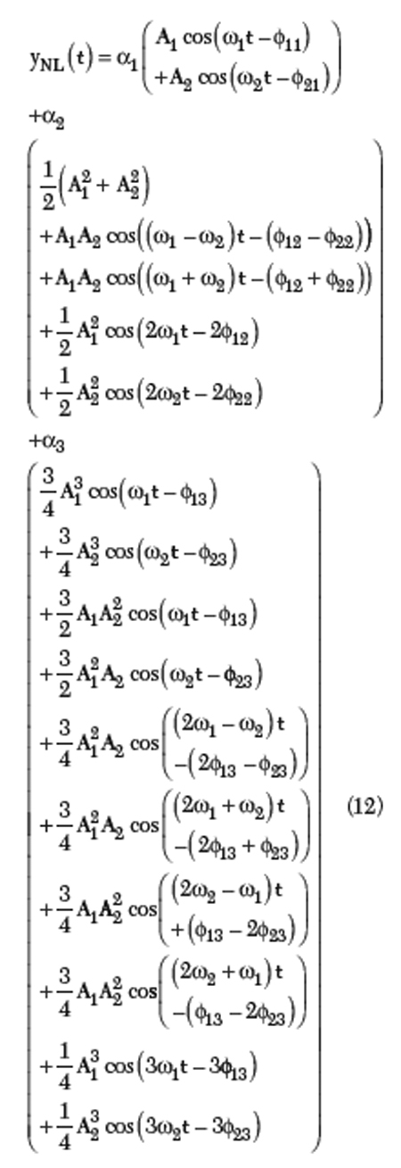
From Equation 12 it can be observed that for a linear system, a sinusoidal input generates a similar sinusoidal response. For the nonlinear model, the response includes second-and third-harmonic distortion terms at 2ωi and 3ωi in addition to the linear term in Equation 10. There is a DC offset term of 1/2 α2A(t)2 that is manifested as a shift in bias from the quiescent point as well as cross-modulation (CM) and intermodulation (IM) products. For example, at the fundamental frequency, ω1 (or ω2), the output can be written as


The first term is the contribution from the linear response, the second is the gain compression or expansion term (AM-AM) and the last term is the cross-modulation term. Table 1 summarizes the classifications of all distortion terms represented above.
Types of Distortion
The distortion products of Equation 12 describe the different components resulting from the effects of a nonlinear device. The distortion products that directly impact the fundamental frequency or frequencies of the input signal cause ‘in-band’ distortion and can be the most challenging to alleviate. Other products describe ‘out-of-band’ distortion that can often be filtered out. The harmonic responses are examples of ‘out-of-band’ distortion.
AM-AM Distortion, AM-PM Distortion and the Error Vector
AM-AM distortion comes from the nonlinear relationship between the output amplitude of the fundamental and the input amplitude at a particular frequency regardless of whether a system displays memory effects. AM-PM distortion is only seen when a system demonstrates memory effects. Examining the contributions of the two-tone response at ω1 gives
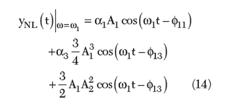
The first term is contributed by the linear response to the input, the second and third terms modify the amplitude and the phase of the linear term. The second term is the result of the input amplitude at ω1 and is the AM-AM and AM-PM term. The third term is the third-order response to the second tone at ω1 and is the cross-modulation term. Since the terms are evaluated at a particular frequency, Equation 14 may be represented as a vector sum as


In the case of a system with no memory, that is, one that has no energy storage elements, there is no phase shift and φ11 = φ13 = 0. The distortion terms modify the magnitude of the linear term and there is no impact on phase. The vector sum becomes merely a sum and the distortion terms either decrease (gain compression) or increase (gain expansion) the linear term depending on the sign of a3. The response at ω1, shown in Figure 1, becomes

Note that in the response to a two-tone input, the AM and CM distortion terms sum regardless of the system having memory. Without memory the angle between the AM and CM vectors is zero and there is no phase distortion. With memory the AM and CM vectors are separated by a non-zero angle and create phase distortion. The AM at ω1 increases or decreases with A13, the amplitude of the first tone cubed, whereas the contribution from the CM term at ω1 grows linearly with A1 but also grows as the square of A2, the result of the cross-modulation from the second tone. The error vector is the difference between the linear term and the sum of the AM and CM terms. In systems with no memory the error vector has no phase and is simply the magnitude of the error.
For systems that exhibit memory effects, the phase of the error term obviously has an impact on the response. To illustrate this, Equation 15 is rewritten as

The error vector magnitude (EVM) is


at an angle of φ13. The angle φ11 is set equal to zero and the vectors are shown in Figure 2. In Figure 2(a), the linear response is plotted on the horizontal axis. The fundamental vector is the resultant of the linear vector and the error vector and has an angle θ. In Figures 2(b) and (c), the effect of increasing and decreasing the amplitude, A1, is demonstrated. The amplitude and phase of the fundamental output signal changes with A1 as does the EVM. AM-AM distortion is often defined for a single-tone input. Then Equation 18 reduces to

Staudinger 5 describes the impact of AM-PM conversion on the PA response and shows the IM products are particularly sensitive to phase distortion. Here, just the impact on the fundamental has been considered.
Harmonic Distortion
The second-harmonic distortion is defined as

which for small distortion, where signal compression or expansion is considered negligible, can be expressed as 6

Similarly, the third-harmonic distortion is defined as

and for small distortion is expressed as

A single-tone applied to the nonlinear system will cause new spectral components to be generated. The output consists of the fundamental and harmonics and demonstrates the phenomenon of spectral regrowth. However, amplifier linearity is more often assessed with the two-tone test.
Intermodulation Distortion: AM-AM
In-band intermodulation distortion (IMD) is a result of the odd-order nonlinearities of a system. From Equation 11, it can be observed that there are distortion terms at ω1–ω2 and ω1+ω2. These distortion terms are called the sum and difference second-order intermodulation distortion (IM) terms. The second-order IM products are not in the band of interest in most communications systems, and IM products and harmonics that are out of band can be filtered out. As before with small-signal levels, higher order terms can be neglected, noting that there are higher order sum and difference terms. The amplitudes of the two-tones are set equal and the magnitude of the third-order IM is compared to the magnitude of the second-order term.
Equation 11 is rewritten as
yNL(t) = α1A(cos(ω1t) + cos(ω2t))
+ α2A2(cos(ω1t) + cos(ω2t))2
+ α3A3(cos(ω1t) + cos (ω2t))3
(24)
The second-order intermodulation is

Thus, when the distortion level is low, IM2 grows proportionally to signal power.
Expanding the third-order term in a similar manner

Equation 26 includes a fundamental term that may cause gain compression or expansion, a third-order harmonic distortion term and a sum term that is generally outside the band of interest but that will be close to the third harmonic term. The last term in Equation 26 is the IM term that will appear in the frequency range of interest. The expression for the IM3 is

Cross-modulation
Cross-modulation occurs when the amplitude modulation is transferred from one carrier to another by nonlinearity in a circuit. The input consists of two tones or more and the level of cross-modulation present in a system is usually determined with two input signals, one modulated and one non-modulated as in
xi = A1cos(ω1t) + A2(1+mcos(ωmt)) cos(ω2t) (28)
where
m = modulation index of the modulated signal ωm = modulating frequency
The amount of amplitude modulation transferred to the signal of frequency ω1 as it passes through the nonlinear circuit determines the cross-modulation for that circuit. Substituting Equation 28 into the power series of Equation 3 yields
y0 = α1(A1cos(ω1t) + A2 (1+mcos(ωmt))cos(ω2t)) + α2(A1cos(ω1t) + A2(1+mcos(ωmt))cos(ω2t))2 + α3(A1cos(ω1t) + A2(1+mcos(ωmt))cos(ω2t))3 +… (29)
Expanding the second term in Equation 29 gives
α2A12cos2(ω1t) + α2 A1A2 (1+mcos(ωmt))cos ((ω1±ω2)t) + α2A22(1+m2cos2(ωmt) + 2mcos(ωmt))cos2(ω2t) (30)
Since cross-modulation results in a term in the form of K(1+δcos(ωmt)cos(ω1t)), it is seen, by inspection, that the second-order nonlinearities do not add to the cross-modulation of a nonlinear system. Cross-modulation contribution from the third term in Equation 29 is

The term 3α3A1A22mcos(ωmt)cos(ω1t) in Equation 31 contributes to cross-modulation (the term involving cos2 (ωmt) does as well but is neglected by convention). Combining the linear term in Equation 29 with Equation 30 in Equation 31 shows that the component of the output at frequency ω1 has modulation at frequency ωm transferred to it

Cross-modulation is defined as

From this it can be seen that CM is independent of A1 and m, and depends only on A22. Equation 28 is valid for small distortion in all applications. If A1 = A2, then

where yom is defined as yom = α1A1
Adjacent Channel Leakage Ratio
Adjacent channel leakage ratio (ACLR) is a measure of intermodulation distortion in wireless transmission systems. ACLR describes the leakage of power from one channel to an adjacent channel. It is an extension to the simple two-tone intermodulation test and quantifies how much of a signal spreads into the next channel. ACLR is the ratio of the total integrated power in the channel adjacent to the signal band to power in the signal band itself 7

In Equation 35 So(ω) is the power spectral density function of the in-band output power.
Conclusion
In this article a polynomial input-output model has been described along with various figures of merit for communication systems. It has been shown how this polynomial model can be used to demonstrate the impact of various distortions on the communications signal. Several typical descriptions of distortion have been described and their impact on the signal has been illustrated.
Acknowledgment
The authors would like to thank Dr. John Wood for his insightful comments during the preparation of this article.
References
1.Federal Communications Commission: Spectrum Policy Task Force, “Report of the Spectrum Efficiency Working Group,” November 15, 2002.
2.J.C. Pedro and N.B. Carvalho, Intermodulation Distortion in Microwave and Wireless Circuits, Artech House, Norwood, MA, 2003.
3.J. Vuolevi and T. Rahkonen, Distortion in RF Power Amplifiers, Artech House, Norwood, MA, 2003.
4.L.O. Chua, C.A. Desoer and E.S. Kuh, Linear and Nonlinear Circuits, McGraw-Hill Inc., New York, NY, 1987.
5.J. Staudinger, “A Consideration of Phase Distortion in Linear Power Amplification of QPSK and Two-tone Sinusoidal Stimuli,” Proc. Wireless Communications Conference, 1997, pp. 105–109.
6.R.G. Meyer, “Course Handouts & Readings, Advanced Integrated Circuits for Communications,” UC Berkeley, 1999.
7.N.B. De Carvalho and J.C. Pedro, “Compact Formulas to Relate ACPR and NPR to Two-tone IMR and IP3,” Microwave Journal, Vol. 42, No. 2, 1999, pp. 70–84.