
Advances in modern radar systems include specialized active antennas, microwave circuits and devices, agile beam steering and shape and digital space-time signal processing. While the pace of radar technology continues to march forward, two fundamentals remain constant. The first is that the electromagnetic properties of antennas, radomes and the installation platform are governed by the underlying and unwavering physics. The second is that engineers designing these systems will push the limits of simulation, based on that underlying physics, to solve ever-larger and more complex electromagnetic radiation and scattering problems. While the physics does not change, the numerical methods engineers and scientists apply continues to advance, built upon the fundamental principles and theorems of electromagnetics.
The technological needs of the radar system designer or antenna designer are to provide understanding of the radiation and scattering performance. A phased array radar antenna, for instance, does not operate in free-space. On the contrary, it may be mounted on the front or side of an aircraft. That aircraft is likely constructed of both metallic and composite materials. The antenna is covered by a radome that likely contains a frequency selective surface (FSS). Understanding the radiation and scattering performance of such a system requires a very comprehensive simulation capability.
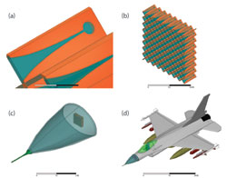
Fig. 1 Components of a phased array radar system include many parts, such as (a) flared notch antenna element, (b) flared notch array, (c) antenna in radome and (d) aircraft platform
Performance of the system and interaction among the various components and subsystems are often not discovered until expensive production of prototypes and testing in the integration lab. What is needed is a full system solution that allows engineers to assemble complex 3D systems and predict system performance and electromagnetic effects using the appropriate global and local simulation technology. Figure 1 depicts a typical phased array radar antenna system. Within that system there is an individual antenna element (flared notch or Vivaldi) assembled into an array. The array antenna is mounted within an aerodynamic radome, which itself may have a FSS applied within its surface. Finally the radar system itself is mounted onto an aircraft.
Numerical Techniques
Modern electromagnetic simulation must handle 3D systems that are physically complex, have a large range of physical dimensions and are assembled based on models from disparate sources, which can include multiple 3D CAD and 2D layout design tools. In addition, it is highly likely that no single electromagnetic simulation technique (such as, Finite Elements, Method of Moments, Physical Optics) can solve the entire system to a desired level of accuracy. A proper and efficient solution requires the ability to apply the appropriate solver technology in a particular area(s) of the system.
Modern simulation methods available in ANSYS® HFSS™ take advantage of advanced computing hardware and novel numerical methods. High Performance Computing (HPC) methods allow large electromagnetic problems to be distributed across a network of computers (cluster) to solve large 3D volumetric problems, to perform material and geometry parametric sweeps, and to solve across frequency. A particularly interesting technique, the domain decomposition method (DDM),1 divides a finite element problem into multiple domains, each of which is then solved on a different computer in the cluster allowing truly massive simulations to be performed.
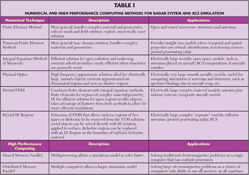
Table 1 provides a summary of numerical and computational techniques available in HFSS that can be leveraged by the design engineer and analyst to solve challenging electromagnetic simulations. The most general technique is the finite element method (FEM) that can solve virtually any geometry shape with complex materials and microwave ports/excitations. The transient (time-domain) FEM offers the additional benefit of providing temporal and spatial behavior of fields especially useful for identifying scattering centers. Other methods like the integral equation (IE) method and physical optics (PO) allow efficient simulation of much larger structures, especially those that are mostly metallic. Both use a surface mesh rather than the volume mesh used in finite elements. The IE method explicitly solves for the electrical current on each surface mesh element. Models that are primarily large surfaces are solved very efficiently using IE. PO is a high frequency (asymptotic) method where currents are approximated on illuminated surfaces of the model and set to zero in shadow regions. Necessarily the model must be illuminated by an external source, such as a plane wave or from a FEM or IE simulation. Typically a PO solver permits only first order interaction (single bounce). The beauty of the PO solver is that it can solve very large models quickly and hence provides quick performance estimates of electrically large problems.
While each of these methods is valuable as standalone solutions to radar antenna and scattering, an even more powerful solution may be had by combining the techniques in a “hybrid” solution. Some portions of a problem are best solved by FEM; other portions are best solved using IE or PO. For instance, the antenna aperture may include Vivaldi radiators with suspended stripline feed elements. FEM is ideal for solving that geometry for radiation and scattering. Once the antenna is placed in a radome, the IE method can be used to compute the Fresnel diffraction and refraction through the radome. In a hybrid technique, the entire problem is solved efficiently by using FEM for the antenna aperture and IE for propagation to and through the radome.
Radar Antenna Systems
Finite-sized Phased Array Analysis
Modeling large, finite-sized phased antenna arrays are an extremely challenging simulation problem. Somewhat by definition these will be electrically large structures with complex geometries. No matter what technique is employed an explicit or a direct solution to the problem will be computationally expensive as the number of mesh elements, matrix unknowns and potentially the number of right hand sides (RHS or excitations), must be large.
The traditional approach for simulating large phased arrays approximates that behavior by assuming an infinitely large array. In such an approach, only the geometric description of a single unit cell is required. Then using a periodic boundary approximation approach a solution for this single unit cell can be developed assuming it is placed in an infinitely large array. Such infinite array analysis has been the staple of antenna array design where the solution for this single unit cell is multiplied by an array factor to determine an approximate behavior of the finite sized array. The approximate nature of this infinite array solution is a result of the fact that the environment, fields and coupling experienced by individual elements of the array vary according to their location in the array (interior, edge, corner, etc.). Lacking this element-level knowledge introduces challenges in finite-sized array design. The design of a corporate feed cannot assume that the active S-parameters of all elements are the same and has to allow for sometimes significant differences especially at the edges of the array. This effect can be mitigated by implementing a band of passive or “dummy” elements around the perimeter of the array. These would allow for the corporate feed of the active elements to assume a more equal input, but would obviously require a larger footprint for the array.
Figure 2 depicts a 256-element array of dual-polarized Vivaldi antenna elements. This array was simulated using two techniques. The first is a new DDM approach2,3,4 that has been developed to effectively and efficiently model finite-sized arrays using distributed memory. The second is a direct solution using a single machine of high capacity as the baseline for computational effort.
Fig. 2 256-element phased array of cross-polarized Vivaldi elements.
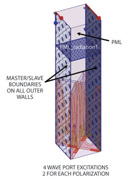
Fig. 3 Unit cell set-up for finite-sized array analysis using DDM.
Figure 3 shows the single unit cell used to simulate the array. The unit cell of the antenna array, including its automatically adapted mesh developed in a periodic boundary condition analysis, is virtually duplicated into the 256-element array geometry. The unit cell and its duplicates are each treated as individual domain solutions for a DDM solution to the entire finite antenna array. The electromagnetic interface between the individual cells is captured by a Robin transmission condition applied on the transverse faces of the cells. Also a continuous conformal tetrahedral mesh is effectively maintained across this interface through a master/slave mesh technique for the unit cell where an identical triangular mesh is enforced on parallel faces of the unit cell.
The calculation of the element domains can be simplified by exploiting the repetitive nature of the elements matrices, A, in the Ax=b calculation for each individual cell. However, not all cells of the array have the same matrix as edge and corner elements reside in a different environment depending on how the elements of the perimeter are terminated and thus corner elements and elements along an edge each have distinct A matrices. Ultimately, to describe a rectangular array, nine unique parent elements are required, one interior plus four edge and four corner. After the matrices for the individual cells are constructed, their solutions collectively become a pre-conditioner for an iterative solution process for the entire system performed at a host node. With this technique, the finite nature of the array, including edge effects, are captured since a unique set of fields are computed for all elements. In addition, this technique is highly parallelizable as the individual units cells can be analyzed across distributed computing cores.
Figure 4 shows results from the analysis. As can be seen in the figure, the element pattern is highly dependent upon the element location in the finite-sized array. A direct simulation of the array required 211 GB RAM and over 122 hours to complete on a single machine. The new DDM simulation required 48.2 GB total RAM and 30 hours computation time on a cluster of 13 machines. That is 77 percent less RAM and 4.1 times faster.
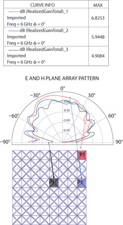
Fig. 4 Array element pattern depends upon location in the array.
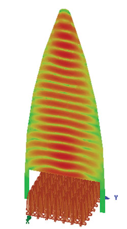
Fig. 5 Simulation of a 256-element Vivaldi array placed within an aerodynamic radome.
Antenna in Radome
Once simulation and optimization of the array has been performed, the next simulation challenge is to observe array performance when placed within a radome. Figure 5 depicts the electric field due to a simulation of the 256-element array placed in the radome. This simulation was performed using a hybrid solution technique that combines FEM with the IE method. The Finite Element Boundary Integral (FEBI) method allows the fields to be truncated into an absorbing boundary created by the boundary integral (BI) surface mesh. In Figure 5, the BI surface mesh is skin-tight up against the outer surface of the radome. Finite elements are used to solve the array and within the radome; the integral equation method is used to solve for the fields exterior to the radome.
Platform RCS
Both the IE and PO methods are popular for RCS computations of electrically large models. Figure 6 shows a comparison of monostatic RCS using the IE and PO methods for an electrically large “cone-sphere” model simulated at 9 GHz (note that for incident radiation toward the tip, the PO model has illumination on the cone due to shadowing). The model has radius = 2.947 inches (diameter = 4.5 wavelengths); length = 23.821 inches (18.15 wavelengths). As can be seen in the figure, the two simulation methods agree very well on broadside incidence near 82 degrees. The PO solution is in very good agreement for all angles but for near incidence on the tip (0 degrees) and for near incidence on the sphere (180 degrees). Creeping wave effects are not accounted for in the PO solution. This becomes apparent as incident angles approach the tip- and sphere-side of cone-sphere.
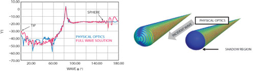
Fig. 6 Comparison of IE and PO solution for monostatic RCS of an electrically large "cone-sphere" model.
While that discrepancy may be important when ultimate accuracy is desired, the entire story is only told when we examine the computational resources required for each solution. When computing the RCS of the cone-sphere, using the IE and PO methods, the PO solution is roughly eight times faster, thus providing a rapid examination of the solution. This performance can be useful when first exploring a design and/or when optimizing a design. It can also be useful in more challenging computations of RCS of real targets, such as aircraft.
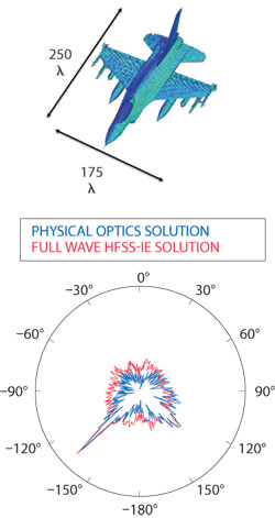
Fig. 7 Bi-static RCS of a full-sized fighter aircraft at 5 GHz computed using IE and PO. Incident wave impinging on target from ϕ = θ = 45 °. (a) Model with induced current (b) Bi-static RCS computation along ϕ = 45°.
The bi-static RCS of a full-sized fighter aircraft at 5 GHz is depicted in Figure 7. The aircraft is electrically large: 250λ by 175λ. The bi-static RCS was computed using both the IE and PO techniques. Of course, the IE simulation was quite computationally intense and hence an HPC solution was invoked. The large-scale simulation was so large that it was only possible using a computer cluster of 10 networked machines. The distributed IE solution used 32 GB of memory on each of the ten machines for a total of 325 GB. Solution time was 33.5 hours total. This rigorous solution provides a highly accurate computation of the true RCS of the aircraft in all regions, including the non-specular directions. To compute the bi-static RCS using PO, the simulation requirements were very modest, only 20 minutes elapsed time using 8.3 G RAM. As can be seen in the figure, the RCS computed by PO along the specular is almost exactly the same as the much more computationally intensive IE solution. Engineers should choose the IE method for ultimate verification accuracy. For early computations, optimization and many mono-static cases, the PO technique offers great advantage to solve on a single machine with fast simulation turnaround.
Examining the RCS performance of an aircraft in a particular band in the frequency domain provides the information needed to understand radar performance. Additional information can be had if simulations are performed in both the frequency- and time-domains. As mentioned earlier, time-domain simulations and associated electric field plots provide information as a function of both time and space. This information is particularly useful to understand a radar target’s time “signature.” It is also very important for design and diagnostics to understand the scattering centers of the target and which elements of the aircraft produce the most significant scattering. Figure 8 shows the electric field over a sequence of three instances in time for scattering of a vertically polarized plane wave striking an aircraft. The plane wave impinges upon the aircraft at a 45 degree angle. The first image shows the plane wave interacting with the radome and an associated specular bounce. In the next image, that incident wave begins to interact with the jet engine inlet below the craft; waves can be seen initiating back toward the source. The third image clearly shows the waves continue their propagation back toward the source. Also seen in the third image is scattering from the wing leading edge. The transient analysis can be used to determine precisely which portions of the aircraft are producing significant scattering and especially the undesirable back scattering for low observable performance.
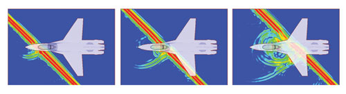
Fig. 8 Time sequence using transient FEM illustrating scattering locations. (a) Initial plane wave. (b) Plane wave interaction with engine inlet. (c) Scattering from engine inlet propagating back toward source. Note also in (c) the scattering off leading edge of wing.
Conclusion
With new technologies, such as IE, hybrid FEBI, IE-Regions and HPC, engineers can solve electrically large full-wave EM models which could not be handled before. Hybrid solutions bring forth the power of specific numerical methods and allow simulation of modes containing regions of complex materials and geometries with outer regions that are electrically large. PO methods provide fast approximate solutions for large metallic models often found in antenna placement and RCS applications. Transient solutions allow engineers to examine the behavior of radiation and scattering in time and space. The physical laws that govern the behavior of radar systems are unwavering. Likewise, engineers will relentlessly drive toward solving ever-larger and more complex electromagnetic radiation and scattering problems. There are equally driven researchers, engineers, and computer scientists committed to expanding the numerical methods and techniques that efficiently solve the challenges of modern radar systems.
References
1. “HFSS™ 12.0: High Performance Computing,” Microwave Journal, Vol. 52, No. 11, November 2009, pp. 118.
2. S.C. Lee, M.N. Vouvakis and J.F. Lee, “A Non-Overlapping Domain Decomposition Method with Non-Matching Grids for Modeling Large Finite Antenna Arrays,” Journal of Computer Physics, Vol. 203, February 2005, pp. 1-21.
3. M.N. Vouvakis, Z. Cendes and J.F. Lee, “A FEM Domain Decomposition Method for Photonic and Electromagnetic Band Gap Structures,” IEEE Transactions on Antennas and Propagation, Vol. 54, No. 2, February 2006, pp. 721-733.
4. K. Zhao, V. Rawat, S.C. Lee and J.F. Lee, “A Domain Decomposition Method with Non-conformal Meshes for Finite Periodic and Semi-periodic Structures,” IEEE Transactions on Antennas and Propagation, Vol. 55, No. 9, September 2007, pp. 2559–2570.