
Terminology
With microwaves defined, the following is an introduction to some of the basic terminology associated with microwaves and wireless technology, i.e. the jargon and the buzz words used by those in the microwave field. This list will be expanded and further refined as subsequent topics are introduced.
Decibel (dB). dB, a relative term with no units, is a ratio of two powers (or voltages). The decibel value can be positive (gain) or negative (loss). If an output power and an output power of a device (or system) is measured, the log of the ratio of the two taken, multiplied by 10 results in a decibel value for gain or loss. When using voltages, the multiplication factor is 20, since power is proportional to the square of voltage. It represents only how much the power or voltage level increases or decreases. It does not, by itself, provide a measure of the actual power or voltage level. It is valuable in determining a system’s overall gain or loss. For example, a filter with a 2 dB loss, an amplifier with a 20 dB gain, an attenuator with a 6 dB loss and another amplifier with a 12 dB gain, has an overall setup (or system) gain of +24 dB (see Figure 1). The value is found by adding the positive decibels (+32) and the negative decibels (-8), and taking the difference (+24).
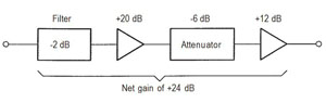
Figure 1 An illustration of decibels.
Decibels Referred to Milliwatts (dBm). Where dB is a relative term, dBm is an absolute number, that is, decibels referred to milliwatts (mW) are specific powers (mW, W and so forth). To determine decibels referred to mW, only one power is needed. For example, given a power of 10 mW (0.010 W), divide it by 1 mW, take the log of the result, and multiply it by 10 (+10 dBm, in this case). The value of +10 dBm means that 10 mW of power are available from a source or are being read at a specific point. That differs greatly from +10 dB, which means only that there is a gain of 10 dB (gain of 10). So, whenever absolute power readings are required, use decibels referred to mW. To help to understand decibels referred to mW and related powers, see Table 1. The table shows five values of decibels referred to mW and the powers associated with them.
| Power | 10 µW | 100 µW | 1 mW | 10 mW | 100 mW |
|---|---|---|---|---|---|
| dBm | -20 | -10 | 0 | +10 | +20 |
The terms decibels and decibels referred to mW can be used together, as illustrated in Figure 2. In the figure, there is an overall gain of +14 dB. One can also see that a +10 dBm signal is applied at the input. Following the decibel and decibel-referred-to-mW levels throughout, one can see that the output is +24 dBm, which is exactly 14 dB higher than the input. Thus, it is shown that decibels and decibels referred to mW can be used together.
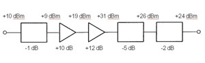
Figure 2 Decibels and decibels referred to milliwatts.
Characteristic Impedance. When thinking of impedance, think of something in the way. A running back in football is impeded by a group of 300-pound defensive linemen; an accident on the freeway impedes the flow of traffic; and alcohol impedes one’s driving skills. All these examples show some parameter in the way of normal operations. A characteristic impedance is an impedance (in ohms) that determines the flow of high frequency energy in a system or through a transmission line. The characteristic impedance most often used in high-frequency applications is 50 ohms. This value is a dynamic impedance in that it is not a value measured with an ohmmeter but rather an alternating-current (ac) impedance, which depends on the characteristics of the transmission line or component being used. An ohmmeter placed between the center conductor and the outer shield of a coaxial cable would not measure anything but an open circuit.[3] Similarly, measuring with an ohmmeter from the conductor of a microstrip transmission line to its ground plane would yield the same result.[4] This should reinforce the understanding that characteristic impedance is not a direct-current (dc) parameter but one that quantitatively describes the system or the transmission line at the frequencies at which it is designed to work.
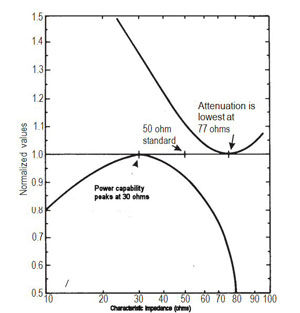
Figure 3 Attenuation and power capability.
As previously mentioned, the characteristic impedance most often used in high frequency applications is 50 ohms. To understand how this value is determined, see Figure 3. It can be seen from this chart that the maximum theoretical power handling capability of a transmission line occurs at 30 ohms, while the lowest attenuation occurs at 77 ohms. The “ideal” characteristic impedance is a compromise between these two values, or 50 ohms. Note also that the characteristic impedance is the same at the input of a transmission line or device as it is 30 cm away, 1 m away, or 1 km away. It is a constant that can be relied upon to produce predictable results in a system.
Voltage Standing Wave Ratio (VSWR). VSWR is used to characterize many aspects of microwave circuits. It is a number between 1.0 and infinity. The ideal value for VSWR is 1:1 (it is expressed as a ratio), which is termed a matched condition. A matched condition is one in which systems have the same impedance, i.e. all energy transmitted by a source travels forward through a transmission media to a load; there is no energy reflected back to the source. To understand the concept of a standing wave, consider a rope tied to a post. If you hold the rope in your hand and flip your wrist up and down, you see a wave going down the rope to the post. If the post and the rope were matched to each other, the wave going down the rope would be completely absorbed by the post and not seen again, i.e. all energy from the wrist is transmitted to the post via the rope. In reality, however, the post and the rope are not matched to each other and the wave comes right back to your hand. If you could move the rope at a high enough rate, you would have one wave going down the rope and one coming back at the same time, adding at some points and subtracting at others. This results in a wave on the line that is “standing still,” which is where the term standing wave comes from.
VSWR is the peak amplitude of the standing wave voltage maximum divided by its peak voltage minimum. It depends on the value of the impedance at the output of a transmission line compared to the characteristic impedance of the transmission line. It also can be shown that the standing wave ratio is a comparison of the impedance at the input of a device compared to the impedance at the output of the device that is driving it. A perfect match is indicated by no standing waves. A drastic mismatch, such as an open circuit or a short circuit, results in a large amplitude standing wave on the transmission line or device. This indicates a very large mismatch between devices or between the transmission line and the load at its output. The larger the mismatch, the higher the VSWR on the transmission line, or at the input or the output of a device. Conversely, a smaller mismatch results in a lower VSWR. The lowest possible VSWR, a value of 1:1 occurs with a perfect match.