
Parametrics and Optimization Using Ansoft HFSS
Ansoft Corp.
Pittsburgh, PA
The high frequency structure simulator (HFSS) is widely recognized as the tool that brought the power of the finite element method to three-dimensional (3-D) RF and microwave design. Finite element analysis allows complicated 3-D structures such as transitions, filters, couplers and antennas to be simulated accurately by computing the underlying electromagnetic fields. Optimetrics™ is a powerful new capability in Ansoft HFSS that speeds the design process and allows users to perform parametric analysis, optimization, sensitivity analysis and other design studies from an easy-to-use interface. With this new capability, dozens of design variations can be performed quickly and effortlessly, components can be optimized to minimize any user-defined cost function and design of experiments studies can be automated to derive sensitivities and uncertainties as a function of manufacturing tolerances.
Optimetrics provides integrated parametrics and optimization capabilities by exploiting the macro scripting language in the simulator. An existing feature of Ansoft HFSS is its ability to record macro commands whenever the software is run. This capability allows any simulator session to be replayed by simply rerunning the associated macro file. Modifying the macros modifies the operations that the HFSS performs and allows quantities such as geometry, materials, boundary conditions, sources and frequencies to be varied.
The smart parametrics and optimization engine in Optimetrics are made possible by having a convenient interface to generate macro commands. At the start of a session, the user creates a nominal problem and defines the independent parameters to be varied. The dependent variables to be computed in a parametric analysis or the cost function to be minimized in optimization is then defined. These dependent variables and cost functions can be of any quantity capable of being computed in the simulator. Field values, S parameters, frequency response, eigenmode data, impedance and antenna metrics are available at the click of a button. The simulator performs the requested computations, providing the output in convenient table format in the case of parametric analysis or in terms of optimal design specification in the case of optimization.
The need for the user to work with the macro commands has been largely eliminated. A user interface has been created that automatically and seamlessly creates HFSS macro commands for most of the operations involved in parametrics and optimization applications. In addition, only a single nominal project is needed, greatly simplifying the input requirements for the user.
Parametric Study
A key feature of Optimetrics is its ability to study performance characteristics with respect to changes in design. Any number of design parameters may be varied in a single nominal project design. In general, geometric shapes, material properties, source excitations, boundary conditions and specified frequencies are independent parameters; S parameters, antenna parameters, eigenmode data or other HFSS-computed quantities are dependent parameters. Users can create compound parameters, which are a function of both dependent and independent parameters. Such a compound parameter can be used for better visualization and understanding of the project or as a cost function to be used in the optimizer. The number of independent or dependent parameters is unlimited. All dependencies, such as boundary conditions, are restored intelligently including face picks, impedance, calibration lines, gap source lines and the UV coordinate system of periodic boundaries. For example, if an impedance line has been created that is one-third wavelength from the end of a port face, this line will always be one-third wavelength for the parametric projects.
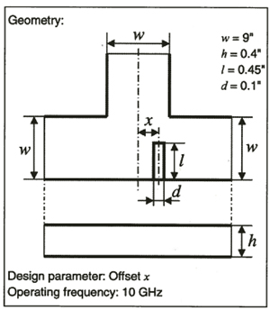
Figure 1 An H-plane reactive T-junction with inductive septum.
Consider the problem of computing the power division produced by an inductive septum in a waveguide T-junction at 10 GHz, as shown in Figure 1. To solve this problem as a function of the septum offset, the nominal problem is entered and solved. With Optimetrics, a table is set up for sweeping the offset with each row of the table corresponding to a specific offset value. (There is no limit on the number of rows users can enter.) Taking into account the parameters specified for the row, solving the table creates an HFSS project for every row of the table. Optimetrics supports automatic seeding for each parametric setup. In the case where no geometry parameter is changed, the refined nominal mesh is used as the starting mesh for all solutions. 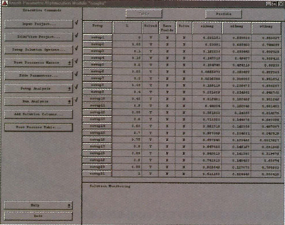 Dependent and compound parameters can be added as columns of a table. In this case, the original dependent parameters of interest are the magnitude of the scattering parameters. Upon execution, the value of the dependent parameter computed for this row's solution fills the far right columns as shown in Figure 2.
Figure 2 Optimetrics table for organizing and simulating parameters.
In this case, the problem size was 8000 unknowns and required three minutes and five seconds per row using a 360 MHz Pentium III processor. If the user is not satisfied with the accuracy of the solution, it is possible to perform additional refinement and obtain a higher accuracy solution for every row. Users can also add frequency sweeps if single frequency information is insufficient.Optimetrics offers users the choice of either saving or deleting the parametric field solutions. Turning off the field-saving feature saves disk space, but the parametric field solutions are not available for later viewing. The values of the dependent parameters are always retained.
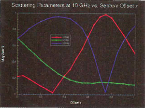
Figure 3 S parameters vs. septum position for the reactive T-junction.
Table postprocessing enables users to plot one column against another, as shown in Figure 3 . Parametric projects can be viewed in the same detail as the nominal project. A macro file created in the nominal project to generate plots can be run for any parametric setup with the click of a button. The saved plots for every row can be plotted together to view the effect of changing parameter values on the plots.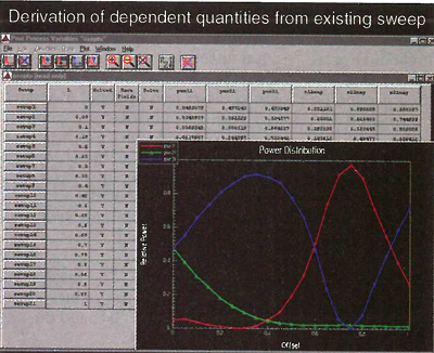 Even after the solution is completed, the user may add new solution columns to the table. In this case, the left-to-right power ratio vs. offset is evaluated and plotted. Within seconds, Optimetrics creates new columns and fills them by deriving the newly requested data from the existing solutions in the corresponding rows. The results are shown in Figure 4 .
Figure 4 New plots of derived quantities.
Optimization
Optimetrics contains a powerful internal optimization algorithm to help users achieve optimal designs. This optimizer employs a constrained superlinearly convergent active set algorithm. To restrict the search region and prevent the optimizer from creating physically meaningless designs (such as overlapping geometry), Optimetrics supports simple bounds as well as linear constraints. The optimized design is guaranteed to be within the feasible domain.
Optimetrics also provides users with unlimited freedom in defining cost functions for optimization. Any algebraic expression may be defined as the cost function and any solution quantity (such as field strength, far-field values or circuit parameters that can be computed in the simulator) may be used as a variable in this cost function. Optimetrics searches the design space to minimize the cost function. To accommodate maximization or compound objectives, the user may construct partial cost functions and/or apply appropriate weights.
To simplify cost function definition for standard tasks, Optimetrics provides a graphical user interface that allows the user access to commonly used quantities (such as circuit parameters) with the push of a button. A special panel for filter optimization is also provided. The user may choose an arbitrary number of frequency bands and specify the requested filter characteristics. Expert users can even create their own macro scripts. The cost functions in the macro script may contain loops and conditional statements.
By default, optimization starts from the nominal settings for the design. However, if a parametric table is available, Optimetrics will first scan the table, analyze all designs that are feasible and start optimization from the design of least cost. Hence, the user may manually create parameter settings for one or more candidates as the starting point for the optimization, or even begin with a parametric sweep. Beginning with a parametric sweep is particularly attractive when the user chooses to inspect the response surface over a wide range of parameters and may also help to avoid local optima.
Fine-tuning a Design
To illustrate some of the productivity gains afforded by Optimetrics, consider the problem of fine-tuning the product design. It often happens that a designer has the basic parameters for a microwave component but needs to fine-tune these parameters to deliver a precision product. Using cut-and-try methods, such fine-tuning can require weeks of prototyping and tweaking; using Optimetrics, it can be performed overnight.
Consider the four-post microstrip bandpass filter shown in Figure 5 . This filter was designed1 in an attempt to meet a design goal of an 8 to 9 GHz passband with less than 1 dB ripple. Using traditional filter design techniques, a filter was designed, fabricated, tested and published with a 7.6 to 9 GHz passband and 1.5 dB ripple. Using the published dimensions as the nominal design, this filter was entered into Optimetrics. The optimization problem consists of four
  parameters: the diameter of the end posts, the diameter of the center posts, the spacing between the end and center posts, and the spacing between the center posts. As shown in Figure 6 , Optimetrics improved this design considerably; the optimized design has a passband from 8 to 9 GHz with less than 0.6 dB ripple, exceeding the design specifications.
Creating a Design from Scratch
In some cases, Optimetrics is able to create an excellent design even though the user has little initial knowledge of a good design. This capability is not foolproof; complex designs often have many parameters and many local minima that can confound direct optimization. A designer is advised to perform a parametric sweep first and must use his or her judgment to create an initial good design. Nevertheless, in some simple cases, the optimizer works surprisingly well in creating designs with minimal user design input.
Consider the microstrip patch antenna in Figure 7 . The design goal for this antenna is to produce an antenna resonant at 2 GHz and the lowest possible  return loss at resonance. The design parameters are the length of the patch and the feed location on the side of the patch. The nominal patch and the optimized patch are shown in Figure 8 ; the corresponding return loss vs. frequency plots are
 shown in Figure 9 . In this case it can be seen that the nominal patch is very far from an acceptable design while the optimized patch provides good performance.
Optimization Using External Optimizers
Since Optimetrics is based on the HFSS macro scripting language, it is possible to drive Ansoft HFSS from start to finish from an outside program. This outside program may be used to adjust design parameters until particular postprocessing results are achieved. The outside program may be written in C, C++, FORTRAN or any other language. Unlike the automated procedures available in an internal optimizer, using an outside computer program for optimization requires a significant programming effort on the part of the user. In the example described here, MatLab™ supplies the optimization algorithm and controls the input to Ansoft HFSS.
Consider the three-element Yagi-Uda antenna shown in Figure 10 . A typical Yagi-Uda antenna should have a high directivity, narrow beamwidth, low sidelobes and a high front-to-back ratio. In this example, the goal was to optimize the variables to achieve a directivity and front-to-back ratio of 8 dB or greater. The antenna consists of a director, driven element and reflector. The distance between the driven element and reflector is denoted by S1 while the distance between the director and driven element is denoted by S2. In order to achieve their functions, the reflector should be longer than the driven elements and the director should be shorter. (Constraints in the optimization were used to enforce these conditions.) Two cost functions were used: one to measure the directivity, the other to measure the front-to-back-ratio. The MatLab multi-objective goal attainment algorithm (fgoalattain.m) was also used.
The cross-sectional radius of the antenna elements is assumed to be 0.003369l (ln l/2a = 5). A search was  performed to determine a combination of element lengths and separation distances such that the directivity and front-to-back ratio are greater than 8 dB. Figure 11 shows the directivity and front-to-back ratio vs. number of iterations. During the first few iterations, the optimizer was able to achieve a
 front-to-back ratio greater than 8 dB, but the directivity was approximately 5 dB. After 34 iterations, the software found its goal at 8.05 and 8.46 dB. Figure 12 shows the initial and optimized dimensions as well as how they changed vs. optimization cycle.
Conclusion
Optimetrics is a powerful new feature in Ansoft HFSS that provides parametric and optimization capabilities for 3-D RF and microwave design problems. The approach used is very general and allows any design quantity to be parameterized and optimized. It even allows outside programs such as MatLab to be used to drive the optimization. The examples shown indicate the ease with which parametric solutions may be set up and the power of the new optimization capability. Significant applications of Optimetrics include fine-tuning preliminary designs, searching the design space for acceptable designs and the possibility of creating excellent designs from scratch. All of these applications provide good productivity improvements for designers and allow precision designs to be created with minimal cost and time.
References
1. MatLab Version 5.3 is a registered trademark of the Mathworks Inc., Natick, MA 01760, USA.
2. K.L. Wu, C. Wu and J. Litva, "Characterizing Microwave Planar Circuits Using the Coupled Finite-Boundary Element Method," IEEE Transactions on Microwave Theory and Techniques, Vol. 40, October 1992, pp. 1963-1966.
Ansoft Corp.,
Pittsburgh, PA
(412) 261-3200.