
Today’s pulse radar systems frequently use pulse compression. This technique combines excellent range resolution and high energy with low peak power levels. For this purpose, the transmission pulse is initially extended in bandwidth and time by intrapulse modulation. A corresponding matched filter in the radar’s receivers compresses the received echo signal in time and increases the peak value by approximately the pulse compression ratio (see Figure 1). This improves the time resolution and thus the range resolution by a factor of the compression. It also reduces the required peak power level, thereby reducing output amplifier and power supply complexity.
Figure 1 Radar system using a digital pulse compression filter.
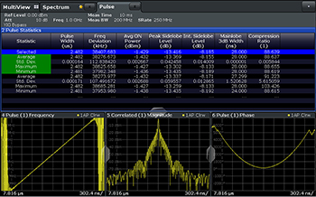
Figure 2 LFM compressed pulse. The correlated magnitude window shows the peak sidelobes are approximately 13 dB down from the peak.
The increased pulse length, however, increases the blind range, and an influence of Doppler on range measurement accuracy can be observed. Furthermore, signal processing in a radar system becomes more complex. Depending on the modulation, the compressed pulse will not only have one narrow peak in time (the main lobe) but will also exhibit
sidelobes, also known as time sidelobes or range sidelobes. These may cause false alarms or appear as a “blurring” of reflections. Despite these disadvantages, pulse compression is widely used today, as the advantages outweigh the disadvantages.
Typical transmission signal types include linear frequency modulation (LFM) or chirp, nonlinear frequency modulation, binary phase-coded and polyphase-coded signals. An example of a binary phase-coded signal is binary phase shift keying (BPSK) with a Barker code. Although more refined techniques have been developed, LFM and Barker codes are still in wide use. In the case of a pure LFM, the compressed pulse shows a sin(×)/× response, and the level of the highest time sidelobe is theoretically 13.2 dB below the main lobe level. This ratio is also known as the peak to sidelobe level (PSL). The PSL represents the ability of a radar system to distinguish between large targets and small targets in the immediate vicinity. Figure 2 shows an example of an LFM compressed pulse with an approximately 38 MHz linear chirp width, together with intrapulse frequency and phase characteristics.
Amplitude weighting, also known as windowing, can reduce the PSL to the required level, but at the expense of a reduced signal-to-noise ratio. In this case, the matched filter is implemented in the digital signal processing of the receiver as a correlation between the echo signal and the ideal Tx waveform. The basic operation, a convolution in time, is most efficiently done as multiplication in the frequency domain, by first performing a fast Fourier transform (FFT) on the received signal, then multiplying the signal by the reference chirp and finally converting it back to the time domain with an inverse FFT. Windowing is well known in FFT signal processing. Commonly used windowing functions are Hamming, Blackman and Blackman-Harris. Table 1 compares the characteristics of these functions. Figure 3 shows the same 38 MHz LFM signal, now windowed using a Blackman-Harris window; the PSL has dropped to –57 dB.
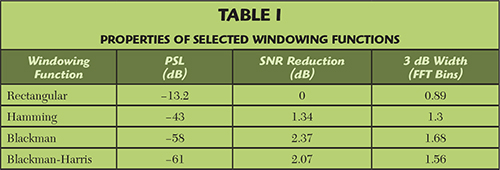
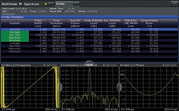
Figure 3 Applying windowing in receiver processing reduces the sidelobe level to 57 dB below the peak.
Measurement Challenges
As soon as a radar uses pulse compression, measuring the pulse width or the rise and fall times is no longer enough for a measurement-based evaluation of the radar’s performance. Any deviation from the desired ideal linear frequency ramp, reflections in the Tx chain, phase and amplitude distortions or modulator inaccuracies will affect the radar’s performance, i.e., its range resolution and range accuracy. The effects can lead to a widening of the main lobe of the compressed pulse and may cause additional or increased time sidelobes exceeding the tolerable level or threshold.
Since LFM, BPSK and polyphase codes are adding modulation to the pulse, one might be inclined to treat this as a communications signal and apply error vector magnitude (EVM) metrics used to measure the quality of communications signals. However, EVM is not easily translated into radar performance parameters such as spatial resolution or false alarm rate. Analyzing the sidelobe behavior directly is therefore the method of choice for evaluating the performance of pulse compression radars. In order to track down sources of performance degradation, this needs to be done at different stages in the signal chain. Using a reference target and looking at the radar receiver processing output is not sufficient. Standard pulse analysis using a measuring instrument (typically a signal analyzer) is necessary, yet not enough. The signal analyzer must also analyze the transmission signal using a suitable matched filter and provide a correlation function, similar to how an ideal radar receiver would operate.
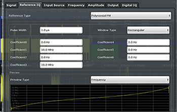
Figure 4 Setting up a reference waveform (matched filter) for a nonlinear FM signal with polynomial coefficients.
As a result of pulse compression, the compressed pulse in the time domain is displayed (see Figures 2 and 3). Any widening of the impulse response (the main lobe) that leads to a poorer range resolution is easy to measure, as well as the sidelobe levels and PSL. Further, frequency error and phase error versus the original pulse length can be shown. In the case of LFM, the frequency error gives a direct measure of the linearity of the frequency ramp.
Many other parameters are used to characterize the compressed signal. With respect to the main lobe, these are the 3 dB width of the main lobe; main lobe power, phase and frequency and the compression ratio. Important measurement parameters for the sidelobes are the PSL, the integrated sidelobe level and the sidelobe delay, i.e., the spacing in time between the main lobe and the closest sidelobe. Main lobe width and sidelobe delay are important system parameters influencing the achievable spatial resolution. Their measurement provides a fast and simple metric to assess the actual spatial resolution achieved in field use. Considering the many parameters that can be used, those most important to the measurement task should be selected. For this reason, any result table should be easy to configure by the user. Figures 2 and 3 show examples of how a signal and spectrum analyzer performs this analysis with its pulse measurement application complemented by a time sidelobe analysis function. The result table has been modified to show only the most important compression parameters. The instrument also provides statistics such as the standard deviation for each parameter, making it possible to assess the stability of the radar signal and the repeatability of the measurement.
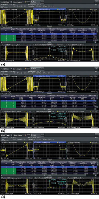
Figure 5 Windowed LFM signal with no I/Q impairments (a) with gain imbalance (b) and I/Q offset (c).
Another concern, besides the correlation function, is the analysis bandwidth or instantaneous bandwidth of the signal analyzer. The bandwidth of the signal analyzer has to cover the bandwidth occupied by the radar’s Tx signal modulation. In the case of a frequency agile radar, the analyzer’s bandwidth should also cover the entire frequency band used for agility. Some signal and spectrum analyzers cover internally up to 500 MHz instantaneous bandwidth. Up to 2 GHz of instantaneous bandwidth can be achieved by using a wideband IF output and digitizing this with a high-performance oscilloscope. In such a case, it is essential that the entire measurement chain, including the scope, be fully characterized for amplitude and group delay distortion. The operator should not need to interact with the signal analyzer and oscilloscope separately, instead operating the system from one point, the signal analyzer.
As the time sidelobe analysis is based on a correlation between an ideal Tx waveform, also referred to as the reference signal, and the measured Tx signal, the first step is to select and create the reference signal. For well known techniques such as LFM, nonlinear FM, Barker-coded BPSK or embedded Barker, it should not be necessary to use additional tools to create this reference; the signal analyzer should create this reference internally. Figure 4 shows an example of how such a reference can be defined, in this case a nonlinear FM signal. For standard LFM, different windows such as Hamming, Hanning, Blackman-Harris, Gauss or Chebyshev should be selectable. Waveforms that are more complex than chirp or Barker codes are used today. Many of them are proprietary or confidential for a simple reason: if the codes are disclosed, a jammer can easily modulate its jamming signal to be compressed like the radar’s own signal and increase the false alarm rate. To account for confidentiality, an analyzer for time sidelobe measurements has to be able to load user-specific reference waveforms as I/Q data.
For example, the R&S FSW features this function and provides tools to easily convert files created in MATLAB to the internal I/Q data format. Techniques where the analyzer captures the ideal reference signal and uses this signal in the measurement are even easier. Visualizing the properties of the imported I/Q data or the captured signal, including amplitude, frequency or autocorrelation, helps users determine whether the data is correctly imported. This technique also makes it possible to compare the waveforms at different stages in the signal chain of the radar and isolate the cause of inaccuracies.
With the time sidelobe measurements well integrated into the analyzer’s functions, the user simply displays the correlated pulse and, if necessary, the frequency and phase error and then adjusts tabular results to provide the parameters of interest. Influences from filters, amplifiers or other radar transmitter components are then easy to identify. Figures 5a and 5b show how an I/Q modulator gain imbalance reduces the PSL from -50 dB to -45 dB. The integrated sidelobe level is reduced even further, from -40 dB in the undisturbed case to -33 dB. An offset on the I/Q modulator will also cause PSL degradation, down from -50 dB to -43 dB (see Figure 5c). The effects can be distinguished by their impulse response as shown in the correlated magnitude display of Figures 5b and 5c.
Notwithstandingthe importance of time sidelobe measurements, the more common pulse parameters — pulse width, PRI, rise and fall times, power, droop, overshoot, ringing, or pulse-to-pulse phase — and their statistics provide additional vital information. Therefore, a universal measuring instrument for radar applications should provide both time
sidelobe measurements and comprehensive pulse analysis. Since the radar’s performance depends on the stability of its oscillators, generally described as phase noise, the instrument should also accurately measure stable oscillators. Advanced signal analyzers provide phase noise measurement functions together with sophisticated pulse analysis, including time sidelobe measurements. They are ideal for many radar systems. To meet highly demanding stability requirements, dedicated phase noise analyzers are commonly used to measure phase noise. The latest measurement capabilities combine ultimate phase noise performance for pulsed signals with signal analysis and pulse analysis capabilities