
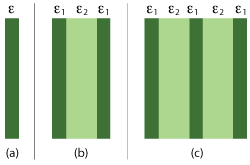
Figure 1 Monolithic radome wall (a), A-sandwich (ε1 > ε2) or B-sandwich (ε1 < ε2) design (b), multi-layered dielectric wall design (c).
Keeping present-day challenges in mind, a complete solution is given for the design and analysis of radomes, from materials characterization through transmission loss analysis, to full 3D radome analysis for calculating radome induced effects. Also discussed is the design and analysis of frequency selective surface (FSS) radomes.
A radome (radar dome) is a structural, weatherproof enclosure that protects a radar system or antenna from its physical environment with minimal impact on the electrical performance of the antenna. Radomes must be radio frequency transparent and therefore constructed of materials that minimally attenuate the electromagnetic signal transmitted or received by the antenna. Selecting a proper radome for a given antenna can improve overall system performance by, for example, maintaining alignment, eliminating wind loading, allowing for all-weather operation and providing shelter for installation and maintenance.1 Radomes find use in a wide variety of applications like satellite, broadcast, weather, communications, telemetry, tracking, surveillance and radio astronomy. Simulation results are obtained using the commercial 3D electromagnetic simulation software, FEKO.2
CHARACTERIZING THE RADOME WALL CONFIGURATION
Radomes, on a broad scale, are classified as monolithic and sandwich designs, based on wall construction as shown in Figure 1.3 There are two types of monolithic designs, half-wave radomes (style-a) and electrically thin-walled radomes (style-b). The sandwich designs can be categorized into A-sandwich (style-c), B-sandwich (style-e) and multi-layered dielectric wall (style-d) radomes. One can also introduce an FSS layer into any of the styles to reduce its out-of-band radar cross section (RCS). The choice of a particular configuration or style depends on the application.
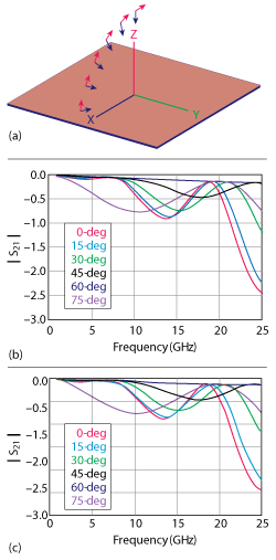
Figure 2 Plane wave incident on the planar Green's function layers at various incident angles (a), transmission loss data computed using Planar Green's Functions (b), published transmission loss results3 (c) for A-sandwich radome.
Transmission loss serves as a key design criterion in selecting wall construction materials irrespective of the radome style. The wall construction material can be used to design a radome of any shape, depending on the application, after characterizing transmission loss. There are several different computational electromagnetic (CEM) methods to determine transmission loss of single- and multi-layered dielectric wall configurations, but the most accurate and efficient is the use of planar Green’s functions with the Method of Moments (MoM).4 The perfect alignment of transmission loss data computed using planar Green’s functions with published results, as shown in Figure 2, validates the accuracy of this method. Transmission loss data is computed for various incident angles over a broad frequency range for an A-sandwich radome, constructed using 0.0762 cm quartz polycyanate skins (εr= 3.23, tan d = 0.016) and a 1.016 cm phenolic honeycomb core (εr= 1.10, tan d = 0.001). The computation time required for these simulations is a nominal 3 seconds, consuming a total of 171 kBytes of memory.
FULL RADOME ANALYSIS
Although transmission loss can be calculated for any incident angle of a planar wall configuration, the shape of the radome introduces other dynamic constraints that change electrical performance. Dissipative losses within the dielectric material, electrical phase shifts introduced by the radome’s presence and internal reflections cause insertion loss, increased antenna sidelobe levels and boresight error.3 It is important, therefore, to analyze radome performance with respect to these additional parameters. The following are various examples of radomes ranging from electrically small to large along with a discussion of CEM methods used for analysis.
Modest-Size Radomes
One can use the full-wave CEM solvers like MoM,5 Finite Element Method (FEM)6 and Finite Difference Time Domain (FDTD)7 for the complete analysis of an arbitrary shaped radome. These full-wave solvers are equally accurate but differ in the computational resources consumed. MoM outshines FEM and FDTD for monolithic and A-sandwich radomes because of the small number of dielectric interfaces in these designs and the fact that an air or free-space volume doesn’t need to be included. As the number of dielectric interfaces increase with multi-layered radomes, FEM being the sparse matrix approximation method, consumes less resources compared to MoM. FDTD has the potential to be the optimal solver for broadband applications, which require solutions over a wide frequency range.
Figure 3 shows a nose cone shaped A-sandwich radome for X-Band applications treated with MoM. The radome profile is built with 0.79732 cm thick skins (εr = 4.8, tan d = 0.0002) and a 3.18972 cm thick core (εr = 1.3, tan d = 0.001). The radome is modest in size with a base inner radius of 1 wavelength and inner height of 1.75 wavelengths, at 9.4 GHz.
Radome induced effects can be calculated by comparing array patterns with and without the radome. One can readily deduce from Figure 3 that the radome introduces an insertion loss of 0.6 dB. There is no shift in the main beam direction which indicates zero boresight error. The sidelobe levels are increased by 5.4 dB, because the signal blockage from the radome reflects RF energy back and reduces the gain. This reflection and retraction of the RF wave front increases sidelobe levels.
Thin-Walled Radomes
A comprehensive radome analysis that explicitly models the dielectric layers is expected to yield the most accurate results. Unfortunately, modeling the physical layers is nearly impossible in scenarios where the overall thickness is much smaller than a wavelength, because the discretization required for the CEM solvers should be comparable to the thickness. However, one can utilize the special formulations that facilitate the analysis of multiple layers of thin dielectric and anisotropic sheets/layers, referred to as the thin dielectric sheet (TDS) approximation.4 TDS replaces all the dielectric layers with one equivalent layer treated with a special impedance boundary condition. The TDS formulation can be used in combination with MoM, where the integral equation (MoM solves the electric/magnetic field integral equations to determine the unknown surface currents) is modified to include the surface impedance of the equivalent dielectric layers.
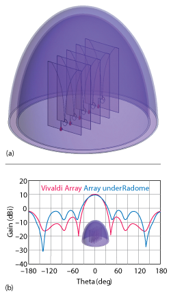
Figure 3 Vivaldi antenna array under a nose cone shaped A-sandwich radome (a), array patterns with and without the radome at 9.4 GHz (b).
The transmission loss data illustrated in Figure 2 indicates that the A-sandwich configuration should be completely transparent to the RF signal at the lower end of the frequency band. A spherical shell radome is built with the same A-sandwich configuration and analyzed for radome induced effects. Figure 4 shows the radome protecting a dipole array. This radome is treated with the TDS approximation as the overall thickness of the 3-layer radome wall is much smaller than a wavelength at the lower end of the frequency band (more specifically at 2.35 GHz).
The gain patterns with and without the radome (see Figure 5) demonstrate that the A-sandwich configuration introduces minimal insertion loss, analogous to the data in Figure 2. The gain pattern also indicates negligible boresight error as there is no shift in the main beam direction.
Moderate Size Radomes
As the electrical size of radomes increase, standard full-wave solvers (e.g., MoM and FEM) require significant computational resources. The multi-level fast multipole method (MLFMM)8 overcomes this challenge by the accelerating MoM solver with fewer computational resources. MLFMM tremendously reduces the computational resource requirements when applied to geometries measuring multiple wavelengths in size. The most appealing aspect of MLFMM is the preserved accuracy, which is governed by a user-controlled residual. In addition, MLFMM can be hybridized with FEM.
Figure 6 shows an ogive shaped A-sandwich radome protecting a dipole array. The electrical size of the radome at its operating frequency of 8.5 GHz is 4.5 and 16.5 wavelengths for base inner radius and inner height, respectively. MLFMM is the optimal solver for the analysis of this electrically large radome. The A-sandwich configuration is constructed with 0.24 cm thick skins (εr = 4.8, tan d = 0.0002) and a 0.4 cm thick core (εr = 1.3, tan d = 0.001). The layers are explicitly present in the simulation (the TDS approximation was not used). The antenna array under the radome is mechanically tilted to point at a 10° elevation angle.
The radome induced effects are illustrated in Figure 7. The A-sandwich ogive introduces a 2.3 degree boresight error and a 1.1 dB insertion loss. Note that the radome design leaves the antenna sidelobe levels intact.
Electrically Large Radomes
Applications such as satellite communications and airborne weather radar require huge radomes to protect the electrically large antennas. The computational resources required to analyze these large structures could become prohibitively large with the aforementioned solvers. One must therefore use asymptotic solvers, particularly Ray Launching Geometrical Optics (RL-GO),9,10 which are efficient when modeling the transmission of rays through objects, like radomes or lenses.
Figure 4 Dipole array under the spherical shell A-sandwich radome, treated with TDS approximation.
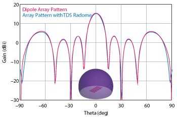
Figure 5 Dipole array patterns, with and without the radome, at 2.35 GHz.
Figure 8 shows the nose cone of an Airbus A380-800 passenger aircraft, which usually covers the weather radar that operates in X-Band, typically at 9.4 GHz. A slotted waveguide (SWG) array, illustrated in Figure 9, is the most popular antenna for the weather radar. The SWG array is designed in such a way that it is fed from the bottom with a single waveguide that is orthogonal to the array waveguides. The length, width and spacing of the slots is optimized for the desired pointed beam pattern.
Figure 6 Dipole array under an ogive shaped A-sandwich radome (a), radiation pattern of the dipole array (b).
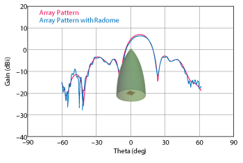
Figure 7 Array pattern with and without the radome.
Aircraft require nose cone radomes that can withstand extreme aerodynamic stresses. For such applications, monolithic half-wave wall configurations are preferred over other styles. Figure 10 shows the transmission loss data of a monolithic wall configuration made of a glass composite (εr = 4.0, tan d = 0.015) with a thickness of 9 mm. The outer surface of the radome wall is coated with a 0.2 mm typical paint layer (εr = 3.46, tan d = 0.068). The material properties chosen for the nose cone radar are obtained from Nair and Jha.11 According to its transmission loss data, the radome performs well over a wide range of incident angles.
Figure 8 Nose cone of Airbus A380-800 passenger aircraft.
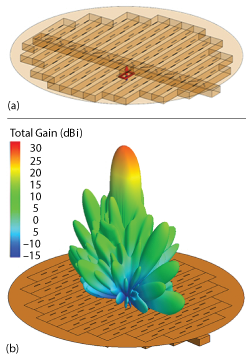
Figure 9 Slotted waveguide array design (a) and array pattern (b).
The weather radar typically scans 60° to 90° on either side of the aircraft heading, while the tilt feature permits the crew to adjust the vertical projection of the beam, typically 10° up or down from the aircraft longitudinal axis. Figure 11 shows the SWG array scanning on both sides of the aircraft. Comparison of its array pattern with and without the radome indicates that a transmission loss of 0.7 dB is introduced because of the glass composite. It can also be observed that the monolithic radome does not introduce any boresight error. The complete analysis of this huge radome is performed using the asymptotic RL-GO method in combination with TDS.
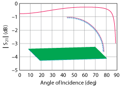
Figure 10 Transmission loss data of a monolithic radome made of glass composite.
FSS Radomes
FSS structures are two-dimensional arrays of periodic resonant elements (printed or slot) designed to either transmit or reflect certain frequency bands. Radomes constructed with slot-FSS layers sandwiched between the dielectric walls act as bandpass filters and reduce out-of-band RCS.12 Transmission loss analysis is also used to characterize the electrical performance of layered FSS wall configurations; however, the planar Green’s function approach becomes computationally expensive as it requires modeling a large finite FSS layer sandwiched between infinite dielectric layers. One can overcome this problem by using periodic boundary conditions (PBC)13 for transmission loss analysis.
PBC analysis requires only a single unit cell large enough to include the FSS element sandwiched between the dielectric layers. The boundary conditions effectively duplicate the unit cell indefinitely, representing the layered configuration as an infinite structure in both dimensions of a 2D plane. This allows for transmission loss analysis of the layered FSS configurations over a range of incident angles. The accuracy of this approach is substantiated by comparison with the planar Green’s function method, which was previously validated with published data. Figure 12 shows a comparison between the planar Green’s functions and PBC approach at various incidence angles for two different wall thicknesses of a monolithic radome (εr = 4.0, tan d = 0.015). The perfect alignment between PBC and planar Green’s function results validates the accuracy of the approach.
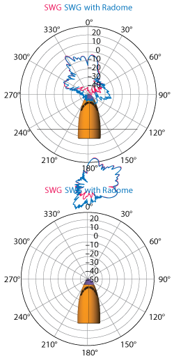
Figure 11 SWG array scanning at different angles on both sides of the aircraft, with and without the radome.
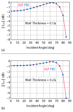
Figure 12 Transmission performance of a thin-walled radome for various incidence angles, comparing planar Green's functions and PBC with wall thickness of 0.1 λ (a) and 0.2 λ (b).
The first step in designing an FSS radome is the selection of a periodic element to meet electromagnetic specifications. A Jerusalem cross-slot FSS geometry is chosen to design an X-Band radome. The FSS layer is placed in the middle of the core layer in an A-Sandwich configuration,1 with 0.319 mm thick skins (εr = 4.8, tan d = 0.0002) and a 1.595 mm thick core (εr = 1.3, tan d = 0.001).
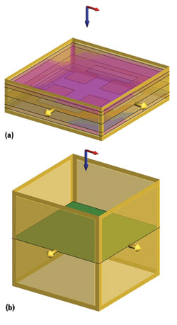
Figure 13 Jerusalem cross-slot FSS layers inside an A-sandwich layered configuration (a), impedance sheet replacing the layered FSS configuration (b).
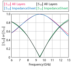
Figure 14 Comparison of transmission and reflection coefficients between the layered configuration with FSS and its equivalent impedance sheet.
Analysis of 3D arbitrary shape radomes with all the explicit layers including the FSS layers is a near impossible task because of the difficulty involved in wrapping the FSS layer onto the curved radome surface. This analysis is simplified by converting the transmission/reflection coefficients of the layered FSS configuration into frequency dependent impedance parameters. One can then replace the explicit layers with a single impedance sheet. This approach dramatically reduces the computational resources when compared with a full analysis of the complete explicit geometry. Figure 13 shows both the layered FSS configuration and its equivalent impedance sheet. The transmission/reflection coefficients of the impedance sheet are compared with the complete A-sandwich layered FSS configuration in Figure 14, validating the accuracy of the impedance sheet approximation. The results also illustrate that the radome is designed to be completely transparent at 9.4 GHz, while exhibiting high insertion loss at both upper and lower frequencies.
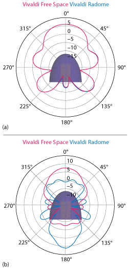
Figure 15 Vivaldi antenna pattern with and without the radome at 9.4 GHz (a) and 12.5 GHz (b).
The radome induced effects are computed through the analysis of a nose cone radome of the above A-sandwich FSS configuration covering a Vivaldi antenna. The Vivaldi antenna patterns with and without the radome (see Figure 15) demonstrate that the radome introduces negligible insertion loss and boresight error at the center of the passband (9.4 GHz). The sidelobe level is also unaffected when operating within the intended frequency band. In contrast, the FSS radome has the greatest rejection at 12.5 GHz, which is consistent with the data in Figure 14.
Conclusion
The computational electromagnetic methods for the complete analysis of radomes ranging from electrically modest to electrically large are discussed with examples. Radome wall construction materials can be quickly characterized for different configurations through a transmission loss analysis using planar Green’s functions and/or periodic boundary conditions. A complete radome analysis to investigate the radome induced effects can be performed using different solvers (e.g., MoM, FEM, FDTD, MLFMM or RL-GO). In addition, a hybridized combination of solvers can be used depending on the electrical size of the radome. The thin dielectric sheet approximation is available for the efficient analysis of thin-walled radomes. A radome with an embedded FSS can be approximated by an impedance sheet with frequency-dependent characteristics. In summary, efficient simulation methods are available for many practical antenna-with-radome applications.
References
- L. Griffiths, “A Fundamental and Technical Review of Radomes,” Microwave Product Digest, May 2008.
- Altair Engineering Inc., FEKO, Suite 7.0, 2014.
- D. J. Kozakoff, “Analysis of Radome-Enclosed Antennas,” Artech House, Norwood, Mass., 1997.
- U. Jakobus, “Comparison of Different Techniques for the Treatment of Lossy Dielectric/Magnetic Bodies Within the Method of Moments Formulation,” AEU International Journal of Electronics and Communications, Vol. 54, No. 3, January 2000, pp. 163−173.
- R. F. Harrington, “Field Computation by Moment Methods,” Macmillan, N.Y., 1968.
- P. P. Silvester and R. L. Ferrari, “Finite Elements for Electrical Engineers,” Third Edition, Cambridge University Press, 1996.
- A. Elsherbeni and V. Demir, The Finite-Difference Time-Domain Method for Electromagnetics with MATLAB Simulations, SciTech Publishing, Raleigh, N.C., 2009.
- U. Jakobus and J. van Tonder, “Fast Multipole Acceleration of a MoM Code for the Solution of Composed Metallic/Dielectric Scattering Problems,” Advances in Radio Science, Vol. 3, January 2005, pp. 189−194.
- H. Ling, R. C. Chou and S. W. Lee, “Shooting and Bouncing Rays: Calculating the RCS of an Arbitrarily Shaped Cavity,” IEEE Transactions on Antennas and Propagation, Vol. 37, No. 2, February 1989, pp. 194−205.
- U. Jakobus, M. Bingle, M. Schoeman, J. J. van Tonder and F. Illenseer, “New FEKO Modeling Capabilities: Waveguide Ports with Dielectrics, Fast MLFMM based Near-Field Calculations, Integrated Network Modeling, and Dielectric GO,” 24th Annual Review of Progress in Applied Computational Electromagnetics, April 2008, pp. 335−340.
- R. U. Nair and R. M. Jha, “Electromagnetic Performance of a Novel Monolithic Radome for Airborne Applications,” IEEE Transactions on Antennas and Propagation, Vol. 57, No. 11, June 2009, pp. 3664−3668.
- C. Sudhendra, A. R. Madhu, A. Mahesh and A. C. Radhakrishna Pillai, “FSS Radomes for Antenna RCS Reduction,” International Journal of Advances in Engineering & Technology, Vol. 6, No. 4, September 2013, pp. 1464−1473.
- J. van Tonder and U. Jakobus, “Infinite Periodic Boundaries in FEKO,” 25th Annual Review of Progress in Applied Computational Electromagnetics, March 2009, pp. 237−242.