
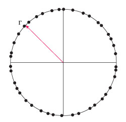
Figure 1 Simulation of reflection coefficient in the complex plane for a constant magnitude Γ.
Amplitude accuracy is a signal measurement challenge that increases with frequency and in many RF and microwave measurements, mismatch uncertainty is the largest single component of amplitude uncertainty. In instrumentation, it is common for only the magnitude of the reflection coefficient to be specified, and for these measurements this article shows how expected mismatch uncertainties may be lower than previously predicted by a factor of three to six. This article shows how a statistical approach, validated by real-world measurements, can yield more accurate uncertainty bounds than commonly used models. Depending on the need, the benefits of reduced uncertainty can yield a tightening of DUT specifications, of course, or can be traded off for improved yield or measurement speed.
Reducing Mismatch Uncertainty:
A Statistical Approach
The effects of mismatch of microwave components are well known to engineers working at these frequencies, and the total effect of the combined mismatches in a system will be a major component of measurement uncertainty. While the general expectation is that the worst case effects due to each element will not add, the current method of setting uncertainty guard-bands is only modestly different from straightforward worst-case analysis.
Most of the industry uses the statistical methods of the Guide to the Expression of Uncertainty in Measurement (GUM).1 This article will describe the authors’ recent work to develop and validate a more accurate statistical model for mismatch uncertainty, and how to use this model to replace older approaches. It is a briefer version of the authors’ longer conference paper2 and will explain the concepts without the mathematical derivation and details. This material is also covered as part of Agilent Application Note 1449-3.3 A convenient way to do the computations is an online spreadsheet.5 The result of using this new model is more accurate estimates of mismatch uncertainty which are three to six times lower than the older methods.
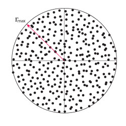
Figure 2 Simulation with Γ is equally likely anywhere within a circle.
Power Delivery and Mismatch
The power delivered to an imperfect power sensor is given by this equation:
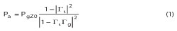
The term PgZ0 is the amount of power delivered to an ideal matched load. The numerator term, 1 - |Γi|2, is accounted for in the calibration of the power sensor. The denominator term, |1 -ΓiΓg|2, represents the mismatch error. If we make the assumption that the cable between the DUT and the power sensor is long, practically speaking we will often not know the phase of the reflections, leading to uncertainty that depends on Γi and Γg.
When we want to combine the uncertainty from the mismatches with other measurement uncertainties, using the method of the GUM, we will usually find the standard deviation of the uncertainty and combine that (a sensitivity-weighted root-sum-square addition) with the standard deviation of other uncertainties; we multiply that by the coverage factor, usually 2, to get the 95th percentile measurement uncertainty. In order to do this, we must have a model of the statistical distribution of the magnitudes of Γi and Γg.
The older literature documents the assumptions of known reflection magnitude and uniform-inside-a-circle reflection coefficients. This article will emphasize a model of Gaussian distribution in the real and imaginary parts of the reflection coefficient, which results in a Rayleigh distribution of the magnitude of the reflection coefficient.
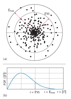
Figure 3 Rayleigh simulation (a) and probability density function (b).
The simplest statistical model, sometimes called the “ring” model, assumes a constant (known) magnitude reflection coefficient with uniformly distributed phase. Classic (and now updated with the information of this article) Application Note 1449-3 from Agilent Technologies3 calls this “case b.” This can be visualized with Figure 1 showing a simulated distribution of the reflection coefficient in the real-imaginary plane.
Because this model is obviously too conservative in many cases, another model has been in use. The “disk” model, shown in Figure 2, assumes that the maximum magnitude is known but the complex reflection coefficient will be equally likely to have a value anywhere within a circle in the complex plane. The effect of modeling both the source and load with the disk model is to give only half as much amplitude uncertainty due to mismatch as for the ring model.
The third model, newly-validated by the research described here, is the “Rayleigh” model, named because the probability density of the magnitude of the reflection coefficient is Rayleigh distributed if the probability density of both complex parts is Gaussian distributed. The simulation is shown in Figure 3a. The simulation figure is annotated with the 95th percentile ring and a “max” ring. These are also shown in the probability density function plot in Figure 3b on a different scale.
Just as the real and imaginary parts with their Gaussian distributions have no true maximum value, neither does the magnitude of the reflection coefficient with its Rayleigh distribution. In order to compare this distribution with the earlier distributions, let us assume that the maximum value given by the manufacturer of the power sensor corresponds to the equivalent of a “3σ” performance level, such that 99.73 percent of manufactured units pass the “max” level and the remainders are not sold.
We can compare the uncertainties of the three models as shown in Table 1.
To summarize: When we know the maximum magnitude of the reflection coefficient of a source and a load, and we assume one of three statistical distributions for that reflection coefficient, and when assuming a Rayleigh distribution, we assume that the “maximum” is equivalent to a “3σ” yield level, the Rayleigh distribution gives an uncertainty six times smaller than the most commonly used distribution for analysis (the ring distribution) and three times smaller than the uniform distribution.
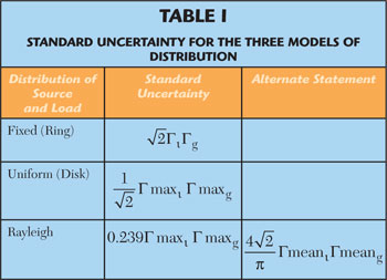
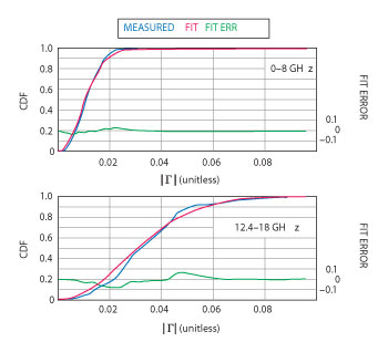
Figure 4 FIT of observations to Rayleigh CDF in two frequency regions.
Evidence and Theory Agree That the Distribution Should be Rayleigh
Theory dates to a 1957 paper by Mullen and Prichard4 that explains how the real and imaginary parts of the reflections of any moderately complex microwave instrument should follow the central limit theorem, yielding a Rayleigh magnitude distribution.
Let us next look at experimental evidence. We will consider three common instruments: a power sensor, a signal generator and a signal analyzer. The authors did their study with the older model 8481A power sensor from Agilent Technologies. The reflection coefficient is specified in the three frequency ranges. For the best and worst ranges, we see plots of the cumulative distribution function (CDF) versus magnitude of the reflection coefficient in Figure 4. The CDF is the integral of the PDF. It is a graphical way of observing the fit that compares distributions without the distractions of using a histogram as the experimental approximation to the PDF. It can be seen that, even for such a simple device as a power sensor, the fit to a Rayleigh distribution is excellent. For a signal source, we see the CDF plot of Figure 5. Finally, one signal path for a signal analyzer is representative of all the signal paths as seen in Figure 6. In all the cases studied, the Rayleigh distribution is an excellent model of the behavior of the instrumentation.
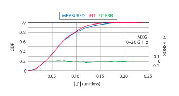
Figure 5 CDF for a signal generator (Agilent MXG).
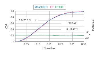
Figure 6 CDF for the high-band preamp path in a signal analyzer (Agilent PXA, Preamp from 3.5 to 26.5 GHz, 0 dB attenuation).
Conclusion
The GUM recommends that measurement uncertainties be estimated as accurately as is feasible. Overestimating measurement uncertainties is a disservice to the users of our products and to our business success. Using the Rayleigh distribution in estimating uncertainty is more accurate than established methods and gives three to six times lower mismatch uncertainty.
References
- Evaluation of Measurement Data – Guide to the Expression of Uncertainty in Measurement JCGM 100:2008 (GUM 1995 with minor corrections), BIPM, IEC, IFCC, ISO, IUPAC, IUPAP, OIML–ISO, Geneva, Switzerland, 2008 (www.bipm.org/en/publications/guides/gum.html).
- M. Dobbert and J. Gorin, “Revisiting Mismatch Uncertainty with the Rayleigh Distribution,” 2011 Conference of NCSL International, August 25, 2011, (http://cp.literature.agilent.com/litweb/pdf/5990-9185EN.pdf).
- “Fundamentals of RF and Microwave Power Measurements (Part 3) Power Measurement Uncertainty per International Guides,” Agilent Application Note AN 1449-3, April 5, 2011, (literature number 5988-9215EN, available online at www.agilent.com).
- J.A. Mullen and W.L. Pritchard, “The Statistical Prediction of Voltage Standing-Wave Ratio,” Microwave Theory and Techniques, IRE Transactions, April 1957, Volume 5, Issue 2.
- “Average Power Sensor Uncertainty Calculator,” Agilent Technologies, April 6, 2011.