
Cables not only transfer the power needed to run electrical equipment, but also the data signals needed to operate them. To prevent errors and device failures, the same attention must be paid to the choice and installation of the cabling as is paid to the rest of the system.
Dealing with data means considering signal integrity (SI). Since data signals are modulated electrical pulses, anything that introduces noise into the cable can corrupt the information, causing equipment to lose performance, malfunction or simply fail altogether. Crosstalk and impedance mismatch are common sources of SI problems; cables generally consist of multiple wires travelling together. The fields generated in one wire can, without proper shielding, couple to others and induce currents in them, while signals can be reflected at the interfaces between cables if the impedances do not match. Analyzing these issues uses RF and microwave techniques and expertise.
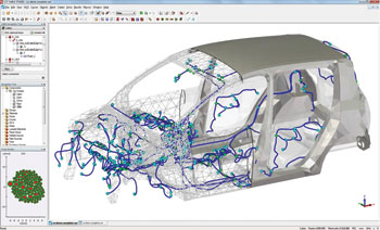
Figure 1 The cabling system inside a car.
It is not just interference from other data signals that one needs to worry about, however. Electromagnetic interference (EMI) can come from a range of sources within the system and the wider environment. Switched-mode power supplies generate noise, while lightning strikes and electrostatic discharge (ESD) introduce transients that often cause damaging current surges in devices. Even the interaction between the equipment and its casing can be enough to interfere with data signals. As well as being immune to external radiation, the cables themselves should not radiate either. Electromagnetic compatibility (EMC) is a legal requirement and this means that they must pose little interference risk to other devices.
Every advance in technology pushes cable design requirements further. High-speed devices demand cables capable of handling ever-higher bit-rates. Automotive and aeronautical systems, increasingly reliant on electronic control and communications systems, need cables that are lightweight yet also measure up to stringent safety regulations. Consumer electronics meanwhile are pushing toward standardized multipurpose cables, where one lead might be used for anything from charging a mobile phone to controlling a printer or transferring data to a hard drive.
In light of these developments, designers have turned to cable harnesses, where multiple cables – sometimes a hundred or more – are tied together and travel along the same conduit as well as hybrid cables, which contain both signal and power wires together. The most familiar example of a hybrid cable is probably USB, but custom cables of many configurations are used in industrial applications. For such complex cable designs, traditional design rules to calculate the cable’s properties become unwieldy. Simulation offers a way to develop and check an arbitrary cable design and optimize its layout and shielding for better performance.
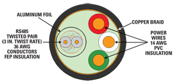
Figure 2 A cross section of a hybrid cable carrying five wires.
Overview of Cable Simulation
Applying full 3D EM simulation methods to simulate detailed cabling within a large structure such as an automobile is impractical, as shown in Figure 1. Each individual wire might be less than a millimeter in diameter, yet tens of meters long, bending as it carries high frequency signals through an electromagnetically complex environment. A conventional simulation of such a system would need an incredibly fine resolution to capture the fields in the cable, extended over a very large volume, resulting in slow, computationally-intensive calculations. The arbitrary cross sections of cables and changes in the surrounding environment along its path make analytic solutions similarly hard to find.
Specialized cable simulators can model complex cables and cable harnesses far more efficiently. The cable can be divided into segments, each having a constant cross-section. A 2D electromagnetic field solver can then be applied to extract the electrical properties for each segment. The properties of the entire cable may be found by cascading the electrical models into an equivalent network. The specialized cable solver may also co-simulate with a full 3D field solver to simulate coupling to and radiation from the cable.
The cable shown in Figure 2 carries five wires – two power wires (red and white), two signal wires (gray twisted pair) and a ground (green). The signal wires are shielded from the power wires by foil and the whole cable is shielded by a copper braid. It is an example of a hybrid cable for which an SI and EMI analysis would be important. The signal wires are not only potentially at risk from external interference, they could also pick up noise from the power wires. The shields and the use of twisted pair wires are both meant to reduce noise in the signal; simulation allows the engineer to investigate their performance. The cable is only a few millimeters wide, but could be meters long.
Line Impedance Simulation
One important property of any data cable is its line impedance. Ideally, the impedance of the data line should match the impedance of the load. If there is a mismatch, signals at the interface between the two will be partially reflected and interfere with the signal, which can lead to SI problems in the connections between the line and components. Reflection is especially problematic for bidirectional cables, where the equipment at both ends acts as both source and receiver.
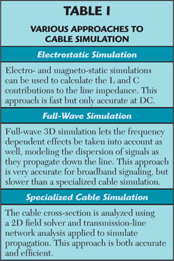
Calculating the line impedance of a cable is an obvious application of simulation. Multiple approaches exist for impedance calculations: the static approach, a full-wave simulation and a specialized cable simulation. Each has its advantages and disadvantages, as shown in Table 1.
A full-wave simulation also permits one to model the connectors at the end of the cable. Impedance matching and EMI analysis are very important when designing or choosing a connector. This is especially true if the connector differs from the cable in some way – for example, if a twisted wire terminates in a straight pin, or if the connector is shielded in a different manner to the cable. The connectors are critical in impedance matching, since they provide the transition between the cable and the load. Often one wants to know which cable dimensions will give suitable cable characteristics to minimize reflection and improve data transmission. To do this, an optimizer is used. The optimizer simulates multiple possible values for model parameters – for instance, the thickness of an insulator or the position of a wire – using sophisticated algorithms to reduce the amount of guesswork involved in finding the best configuration.
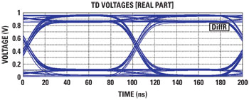
Figure 3 Eye pattern of a 20 m long cable carrying a 10 Mb/s signal.
Calculating Losses
Losses in the cable cause signals to be attenuated, with the degree of attenuation depending on the frequency. High frequencies typically suffer from greater loss, which has the effect of rounding the sharp edges of data pulses, limiting the data transmission rate.
The AC resistance (skin effect) of the wires is one obvious contribution to losses. Another is the loss tangent of the dielectric insulation materials. Signals may also leak through non-perfect shields, introducing additional losses into the circuit. Full-wave and specialized cable simulation both allow designers to calculate the losses for a cable. Full-wave simulations of short cable sections can be cascaded, allowing losses over the whole length to be found without having to solve a full model of the structure.
Simulation can also calculate the scattering parameters (S-parameters), which describe the cable’s characteristics concisely and show how the losses vary with respect to signal frequency. Standard measurements used in the lab such as the eye diagram, shown in Figure 3, can also be replicated with simulation. To produce an eye diagram, a series of random bits are fed into the cable, and the output at the other end captured and graphed. Layering the output signals gives a useful illustration of the rounding of the pulses caused by attenuation.
Crosstalk Simulation
The potential for crosstalk arises whenever two or more wires are coupled. In the example, the power conductors can couple with the signal lines. This sort of broad spectrum noise may be difficult to filter out of signals. Instead, the best option for reducing crosstalk is to shield the wires well and make sure the coupling is minimized.
Since the data is carried by differential signaling, it is the difference between the two wires (the differential mode) that matters. If the cable system is perfectly balanced, the noise coupled to each conductor in the differential pair will be equal and the receiver will be able to reject the noise when the voltage signals are subtracted.
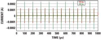
Figure 4 Induced differential mode currents for twist length of 1.5 in. (red) and 3 in. (green) of the hybrid cable, assuming no shielding.
Simulating Twisted-Pair Wire
Twisted-pair cabling, commonplace in communication systems for over a century, winds wires around each other in sets of two. This minimizes the loop area between the wires to reduce mutual inductive coupling. It also helps to maintain balance in the line, equalizing the exposure of each conductor to external fields. Coupling is reduced as long as the twist length is small compared to the wavelength of the interference. The precise choice of twist length can make a big difference to how immune the cable is to crosstalk; for cables carrying several pairs of signal wires, such as the ubiquitous Cat-5, giving each set of wires a slightly different number of twists per meter can reduce the crosstalk between them significantly.
With simulation, the cable designer can examine the interference experienced by the wires and test how different wire configurations affect the signal characteristics. Cable simulation lets one easily adjust the distance between twists (twist rate) in the computer model, and simulate the induced currents caused by switching noise in each case (see Figure 4). For this cable, making the twists shorter makes a big improvement to the differential mode noise rejection characteristics of the line. These simulations are performed without a shield around the twisted pair to study the noise rejection due to twisting alone.
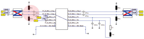
Figure 5 A length of the cable is attached to a lumped element circuit in CST DESIGN STUDIO™. The imbalanced section is highlighted.
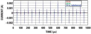
Figure 6 Differential mode crosstalk in the imbalanced system (blue) massively outweigh the crosstalk in the balanced system.
Wire twisting is most effective if the two wires are well-balanced. In a real system, with varying loads and imperfectly manufactured components, this will not always be the case. The cable model can be attached to a circuit made up of lumped elements to replicate the equipment at either end and one can see how well the cable performs when the manufacturing tolerances are taken into account. In this example, shown in Figure 5, a 10 percent imbalance is introduced in the shunt inductance (a drop of 10 µH) and a 4 percent imbalance in the series capacitance (a 20 nF decrease).
This proves to have a huge impact on the coupling. The peak induced current in the imbalanced system is ten times greater than in a perfectly balanced system, leaping from 0.2 to 2 mA – a 20 dB increase in the intensity of the crosstalk (see Figure 6).
Shielding
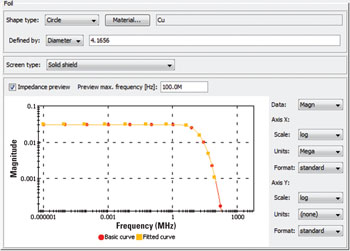
Figure 7 Creation tool box for a foil shield in CST CABLE STUDIOTM, showing the transfer impedance curve over a range of frequencies.
For an extra layer of protection, which should guard against crosstalk and interference even if the cable terminations are not balanced, the wires can be shielded. Different shield types exist for different applications: the main two are foil shields, consisting of a thin sheet of metal such as aluminum, and braided shields, which are made up of many thin wires woven into a tube. Shields can either go around the entire cable to keep out external interference, or they can be placed within the cable to reduce crosstalk.
However, shielding not only adds bulk and weight to the cable, it can also decrease its flexibility and drive up the manufacturing costs. With many types of shielding available, each with different properties and suited toward different types of interference, it is not always easy to balance a cable’s noise characteristics against the design requirements.
The performance of a shield is measured by its transfer impedance, as derived by Schelkunoff.1 The transfer impedance ZT is given by:
where I0 is the current flowing on one side of the shield and dV/dx is the voltage per unit length along the opposite side. The transfer impedance effectively provides a measure of to what extent the shield’s construction prevents fields passing through. The environment does not affect the transfer impedance – it is solely an intrinsic characteristic of the shield itself. The lower the transfer impedance, the better the shielding.
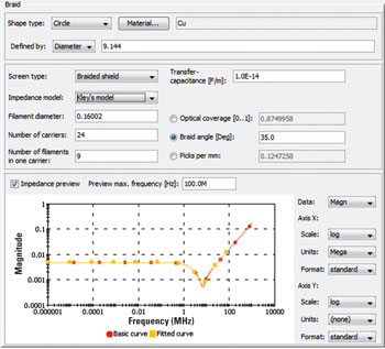
Figure 8 The same dialog for a braided shield. The transfer impedance rises dramatically at high frequencies.
In a foil shield, the skin effect improves shielding performance at high frequencies as shown in Figure 7. Current diffuses through the shield at low frequencies, but is confined to the surface at high frequencies. This means that external fields cannot penetrate the shield at high frequencies, provided that the shield is perfectly closed and has no apertures. However, in a real shield, fields can also pass through the seam formed where the layers of foil overlap, and for a more accurate simulation, this seam can also be taken into account.
Braided shield, by contrast, behaves the opposite way. The transfer impedance of a braided shield, as described by Kley,2 depends on a number of effects. The skin effect still plays a role, but more significant at high frequencies are the small apertures between the strands and the mutual inductive coupling, as well as an inductive interaction, known as “porpoising,” when strands cross each other. These drive up the transfer impedance, so that a braided shield is most effective at low frequencies. Figure 8 shows the transfer impedance curve for a braided shield across the frequency spectrum.
Because mathematical models exist to describe the behavior of shields based on their properties, they are ideal candidates for designing and testing with cable simulation software. Arbitrary shields, whose properties are found experimentally, can also be used in simulations, simply by importing their transfer impedance profile.
If there are multiple shields, their combined transfer impedance can be found analytically by taking into account the internal impedance of each shield and the inductance between them.3 Cable simulation software incorporating such calculations is capable of simulating multi-layer shielding arrangements. Because foil and braided shields work best at different frequencies, combining the two in the cable gives it a good broadband noise rejection profile. The crosstalk analysis can now be repeated, but with shields in place – in this case, either a foil shield or a combined foil and braid shield around the signal wires – to see how this affects the noise characteristics of the cable.
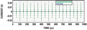
Figure 9 Common mode noise for different shield arrangements. The induced current when both shields are used is too small to see.
The combined two-shield cable has far better coupling rejection than the cable with just a foil shield. In fact, the common mode noise is so low on this cable that it is too small to see in Figure 9– the peak current is less than 4 µA.
The cable and the connector can also be combined together in one simulation. Circuit co-simulation, combining results from multiple full-wave and cable simulations, connects components so they can be simulated as a system. Figure 10 shows a circuit for one such simulation: the power lines are driven by a periodic switching voltage and the load is modeled by lumped elements. The output from the cable – the blue box on the middle-left – is simply linked to the input of the connector from Figure 11– the gray tube on the middle-right. Because the S-parameters of the connector have already been calculated, the circuit solver can run very quickly; there is no need to rerun the entire 3D full-wave calculation.
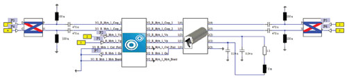
Figure 10 A circuit for testing a cable linked to the load by a shielded connector.
Experimental Verification
As a demonstration of the effects of grounding and shielding on EMC, and to show the accuracy of cable simulation, multiple cables – standard RG58 coax with a braid, RG6 coax with a combined foil/braid shield, twisted pair with a foil and drain wire, shielded twisted pair (STP) with a braid, and the unshielded versions of the cables – had their EMI properties studied, both experimentally and using computer modeling. These cables were terminated in TNC connectors, which contain a metal shell or shield, enabling an ideal 360° connection between the cable and connector shield. To provide a further comparison, an additional length of twisted pair wire was terminated in a non-shielded connector with a “pigtail” connection from the cable shield to the inside of the enclosure housing (see Figure 12).
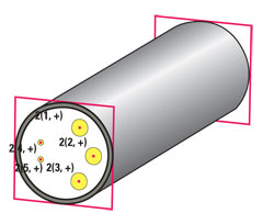
Figure 11 A shielded connector compatible with the hybrid cable showing the ports for simulation.
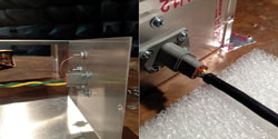
Figure 12 The experimental setup showing the pigtail connector (left) and the signal cable (right).
The interference source was a wire loop radiating across a range of different frequencies. This loop can couple to the signal wires in the cable – the extent to which the cables reject this interference enables the shielding effectiveness to be assessed. The system would be difficult to solve accurately in full 3D due to the small details in geometry and the specialized cable simulator makes it possible to solve the problem in a fraction of the time (see Figure 13).
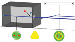
Figure 13 Model of the same system in CST CABLE STUDIO™ showing the wire cross section for each segment.
Figure 14 shows the results of the study, where increasingly negative coupling corresponds to higher shielding effectiveness. The unshielded results serve as a reference. The spiral/drain cable with a pigtail termination provides an additional 20 dB or so of shielding at low frequencies, but its effectiveness degrades at higher frequencies. The same cable was simulated with a TNC termination (dashed blue line) for comparison, and provides further improvement in shielding, as expected. The STP, RG58 and RG6 cables show good shielding effectiveness at all frequencies. Unlike a 360° shield termination, which provides a low impedance connection from the shield to the ground, the pigtail connection adds inductance and the corresponding frequency-dependent impedance. Furthermore, the aperture in the enclosure is no longer closed and may leak electromagnetic fields to the interior of the load box, coupling noise to the exposed signal wires.
The measurements all agree closely with the simulation. With highly shielded cables, the coupling is very small and the induced signals may be below the noise floor of the experimental equipment. This explains some differences for coupling levels below –90 dB. Although it only used a very simple representation of the system, cable simulation was able to model the results very accurately – the simulation even identified a significant resonance at approximately 65 MHz that was subsequently seen in the experiment.
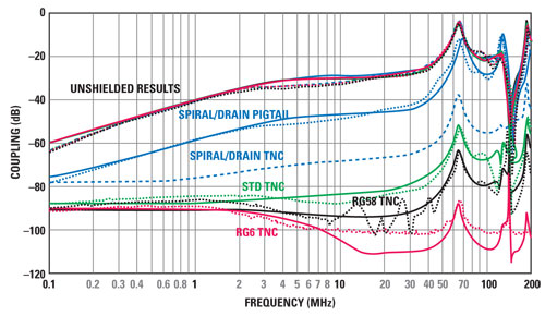
Figure 14 Coupling between the shield and the transmitter for different types of cables, simulated (solid lines) and measured (dotted lines).
Transient Co-simulation
Calculating the properties of a cable gives a good idea of its intrinsic characteristics, but in the real world, cables are rarely if ever completely isolated from the environment. Nearby structures, external fields and the route of the cable can all have an effect on signals within the cable. The transient nature of many interference effects, however, means that a full-wave simulation is necessary to model the precise behavior of many potential sources of interference, such as ESD and electromagnetic pulses (EMP).
Simulation is therefore a useful tool for full system design, but neither specialized cable simulation nor full 3D simulation alone is ideal for giving a complete picture of how a cable behaves in a complex system. Combining them into a hybrid co-simulation task means that the advantages of both – the fast, accurate cable models and the versatility of full-wave – can be brought to the fore.
Two types of cable co-simulation exist: unidirectional and bidirectional. In unidirectional simulation, the cable is assumed to be either a transmitter or a receiver, while in bidirectional simulation, it is both. Bidirectional simulation is therefore most useful for examining how the coupling between a cable and its surroundings affects signals on the cable itself.
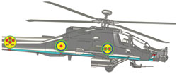
Figure 15 A simple wiring system inside a helicopter, showing cables for the control system, antenna (center) and rotor (right).
Figure 15 shows a typical application of bidirectional co-simulation. The helicopter contains a number of cables, carrying both power and signals, following complex curved routes. The cables may directly couple if routed too closely together, and radiated fields may excite resonances inside the vehicle, which can lead to increased coupling. Transient co-simulation allows a number of different scenarios to be modeled. One example would be the potential susceptibility due to an electromagnetic pulse (EMP). A pulse striking the aircraft may couple to the inside through imperfectly conducting panels and seams inducing current in the cabling.
Conclusion
Simulating cables requires careful consideration. Specialized cable simulation software can be incorporated into the cable design workflow to speed up the process and give the designer an idea of how the cable will behave once connected to the system. These calculations can give not only the electrical properties of the cable itself, but also permit to observe how fields propagate along the cable and interact with the environment. Properly set-up, cable simulations can replicate real-world situations very accurately, with the results of simulations agreeing very closely with measurements in the laboratory or field.
Acknowledgments
The authors want to thank Jeffrey Viel at NTS for providing EMC test facilities.
References
1. S.A. Schelkunoff, “The Electromagnetic Theory of Coaxial Transmission Lines and Cylindrical Shields,” Bell System Technical Journal, Vol. 13, No. 10, October 1934, pp. 532-579.
2. T. Kley, “Optimized Single-braided Cable Shields,” IEEE Transactions on Electromagnetic Compatibility, Vol. 35, No. 1, February 1993, pp. 1-9.
3. E.F. Vance, “Shielding Effectiveness of Braided Wire Shields,” IEEE Transactions on Electromagnetic Compatibility, Vol. 17, No. 2, May 1975, pp. 71-77.
David Johns is the VP of engineering and support at CST of America and is based in the Framingham, MA office. He holds a Ph.D. in Electrical Engineering from Nottingham University UK, specializing in the development and application of the TLM method. He has been actively involved in the modeling of EMC, EMI and E3 problems for over 20 years.
Patrick DeRoy is an application engineer at CST of America and is based in the Framingham, MA office. He recently completed his M.S. degree in Electrical Engineering at the University of Massachusetts, Amherst. His Master’s project focused on cable shielding and transfer impedance modeling using CST STUDIO SUITE and validating simulation results by comparison with measurements.