
In a perfect world, receivers would use brick wall filters, amplifiers and mixers would never distort, command centers would always coordinate their spectrum operations and the term “jam” would have meaning only at breakfast and during musical gatherings. Until then, there will be interference. Interference may be either unintentional or intentional. Whatever the form, the most significant effect is reduced sensitivity in the receiver, potentially disrupting or completely blocking reception of desired signals.
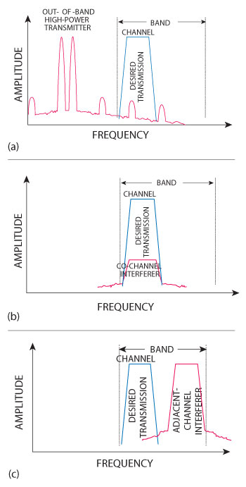
Figure 1 Intermodulation products that fall within the passband (a), co-channel interference (b) and adjacent channel interference (c).
Unintentional interference is often caused by the ever-increasing number of emitters in the RF environment: cell phones, wireless links, cordless phones, terrestrial television and medical electronics are among the many contributors. In addition, some military systems have the potential to cause unintentional interference that disrupts civilian systems ranging from garage door openers and automobile key fobs to Wi-Fi links and the cellular infrastructure. The effects of unintentional interference range from merely annoying in residential settings, to potentially costly in business or medical environments. This type of interference can often be detected, characterized and mitigated through susceptibility and interoperability testing.
In contrast, intentional interference has been created to disrupt the operation of a “victim” receiver. This is undesirable in a wide range of aerospace, defense and public-safety applications: radio communications, radar scans, electronic countermeasures, telemetry links, flight-range operations, spectrum monitoring, signal intelligence and more. On the other hand, intentional interference is a desirable asset when used to block transmissions to improvised electronic devices (IED) or otherwise disrupt enemy tracking, navigation and communication systems. The need to understand and either create or defeat intentional interference is typically exponentially more urgent than interoperability or susceptibility testing.
This article focuses on intentional interference and the ultimate goal of countering undesired signals. The proposed process has four steps: capture the signal in the field, analyze it in the lab, simulate and playback the signal and develop ways to defeat it.
Sketching the Goals of Interference Testing
Unintentional interference from “friendly” systems can be understood by testing for interoperability and susceptibility. Interoperability testing centers on verifying the compliance of a design relative to published standards. It is important to understand how well a system meets its design criteria in the presence of real-world signal levels.
Susceptibility testing focuses on unintended interactions between the system-under-test and other RF systems. In aerospace, military and public-safety, this includes receiver performance in the presence of other mission-critical RF assets. One key goal is to avoid unwanted effects that reduce or block receiver sensitivity during any type of operating scenario.
Outlining the Need for Interference Testing
Various types of “culprit” emitters can affect a victim receiver, and the culprit may be producing out-of-band or in-band interference.
Out-of-band interference is most severe when the culprit is a high-power transmitter operating near the victim (see Figure 1a). The most common problems are passive intermodulation (PIM), RF overload and spurious signals. PIM occurs when dissimilar or corroded metals near large broadcast antennas act as nonlinear junctions (that is diodes). These create intermodulation products that fall within the passband of the victim receiver, reducing its sensitivity. Similarly, harmonics and spurs from a high-power out-of-band transmitter can fall within the passband of the victim and desensitize the receiver. RF overload occurs when electromagnetic energy, regardless of frequency, couples into the receiver’s antenna and front end, thereby desensitizing the victim. As an example, dense RF congestion in a shipboard environment can cause coupling strong enough to physically destroy RF front-end circuitry.
In-band interference comes from other systems that are operating in the same frequency range as the receiver. This type of interference will pass through the victim receiver’s channel filter and, if the signal amplitude is large relative to the expected signal, that signal will be corrupted. Two forms of in-band interference are especially prevalent: co-channel and adjacent-channel. Co-channel interference comes from another transmitter operating in the same spectrum occupied by the victim receiver (see Figure 1b). Although this is common in the cellular industry due to frequency reuse plans, military systems also can experience the same problem, especially in-theater where it may be more difficult to coordinate frequency planning prior to an operation.
Adjacent-channel interference is the result of in-band transmissions that produce unwanted energy or “energy splatter” in channels at higher and lower frequencies (see Figure 1c). This energy splatter, often called intermodulation distortion or spectral regrowth, is created by nonlinear effects in the transmitter’s high-power amplifier.
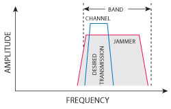
Figure 2 Intentional interference.
Focusing on Intentional Interference
Intentional interference is being transmitted for a specific purpose: disrupting communication, jamming a radar system, and otherwise deceiving or disrupting a victim receiver (see Figure 2). Because such signals are intermittent and transient, it is often difficult to pinpoint the culprit.
Within this scenario, the specific problem is capturing and analyzing a complete set of spectrum data that contains an offending signal. This often requires the acquisition of seconds, minutes or hours of spectrum data — and this can consume gigabytes or terabytes of disk space. To provide a complete picture during analysis, the captured data must be gap-free. In most cases, storage capacity is perhaps the easiest part of the problem. More difficult is the continuous acquisition of high-fidelity RF data. Once the mountain of gap-free data has been acquired and stored, the next challenge is pinpointing one or more interference events. True understanding comes with the extraction of meaningful signal information — in the time, frequency and modulation domains — from each event.
Leveraging Recent Innovations
Advances in commercial off-the-shelf (COTS) technologies are providing the levels of performance needed for effective interference analysis in radar and EW applications. This is true for both the capture and playback of possible interferers.
Driving the Evolution of Signal Analysis
Accurate, gap-free analysis of the RF spectrum requires one or more fast digitizers coupled with excellent front-end circuitry. In a signal analyzer, this equates to exceptional performance that reduces measurement uncertainty and reveals new levels of signal detail. Several key specifications enable the level of performance needed for interference analysis. First is a spurious-free dynamic range of up to 75 dB at a 160 MHz analysis bandwidth. Next are −129 dBc/Hz phase noise (room temperature) at 10 kHz offset (1 GHz), ±0.19 dB absolute amplitude accuracy and sensitivity of −172 dBm displayed average noise level (DANL) at 2 GHz, with a preamplifier and noise floor extension (NFE) technology.
NFE provides a dramatic improvement in a signal analyzer’s ability to accurately measure low-level signals approaching the theoretical “kTB” noise floor. This method compensates for the noise contribution from active microcircuits in the analyzer’s RF and IF chain. With increased averaging, the analyzer’s effective noise floor can be extended by up to 10 dB because 90 percent or more of the contributed noise power is predictable. As a result, that noise is modeled, measured and calibrated during the manufacturing process for all allowed operating conditions the analyzer may face and then eliminated automatically during normal measurements.
Enabling Highly Accurate Signal Scenarios
For playback of captured or simulated signals, the critical attributes of an arbitrary waveform generator (AWG) are bandwidth, accuracy and dynamic range (resolution). These characteristics are especially important in radar and EW applications because today’s typical signals have fast transition times, short on/off intervals and widely divergent power levels. Most typical AWGs require a tradeoff between units that offer either wide bandwidth with low dynamic range or limited bandwidth with high dynamic range. The respective levels of performance in bandwidth and dynamic range depend on the digital-to-analog converter (DAC) used within the AWG. Bandwidth is limited by the DAC sample rate and accuracy is limited by the quality and performance of the analog components used within the device.
A poorly designed DAC may produce glitches that corrupt the spectral content of the output signal, potentially causing inaccurate results. In a typical DAC, nonlinear slewing of the output signals is one possible cause of unwanted signal distortion. This problem is often caused by switched current sources within the DAC. Filtering is typically used to reduce the effect, but this can have an adverse effect on bandwidth.
Interference analysis requires signal generation that is free from the spurs and distortion produced by typical DACs. This is possible with state-of-the-art devices recently developed by Agilent’s Measurement Research Lab. These DACs have two key attributes. First, the device allows switched current sources to settle within the DAC. Second, the DAC re-samples the signal with a special low-noise clock before outputting the simulated signal. This innovation makes it possible to deliver excellent spurious-free dynamic range at wide bandwidths.
Using this type of DAC in an advanced AWG makes it possible to provide high resolution and wide bandwidth simultaneously. For example, Agilent has an RF-quality DAC that provides 14-bit resolution at 8 GSa/s or a 12-bit resolution at 12 GSa/s. Spurious-free dynamic range of less than −75 dBc gives developers confidence that they are testing the radar or EW system, not the signal source.
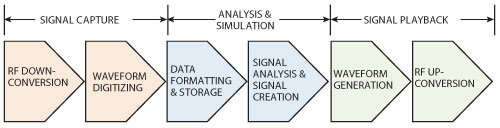
Figure 3 Block diagram of the conversion process of captured interference into useful information.
Structuring the Solution
The driving idea behind the proposed solution is “captured interference equals information.” Quick and accurate extraction of meaningful signal information enables rapid understanding of the interference, its impact on the victim system and possible mitigating countermeasures. All this can be accomplished with a configuration based on COTS hardware and software elements. The system accelerates the process of sifting through terabytes of data and performing detailed analysis. It also retains the original signal fidelity throughout the entire process — capture, analysis, simulation and playback. Because all elements are COTS, the solution offers traceable performance and enables easy redeployment as a conventional test system. An overall block diagram is shown in Figure 3.
Capturing and Analyzing Interference Signals
Signal capture and analysis utilizes three hardware elements: a signal analyzer, a data recorder and an external data pack. These are shown in the left and center sections of Figure 4.
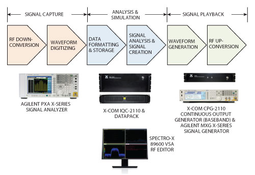
Figure 4 A combination of cots hardware and software elements enables high-fidelity capture, analysis, simulation and playback of interference signals.
Signal analyzer: A high quality signal analyzer is used as the front-end downconverter and IF digitizer. Maximizing signal fidelity at the beginning of the process helps ensure high fidelity through the remaining stages.
High-capacity data recorder: The input to the recorder is a stream of digital I/Q samples from the signal analyzer. The data recorder formats the I/Q data, tags it with external marker events and adds time and GPS stamps before sending to the data pack.
Data pack: The unit used here can be configured with a capacity of 2, 4, 8, 12 or 16 TB.
A variety of post-processing activities can be performed with the software elements of the solution.
Signal analysis software: Key capabilities include pre-processing of large data sets and location of suspect signals. Useful features include built-in search engines to identify and “fingerprint” waveforms as well as “clip and save” capability for replay into vector signal analysis (VSA) software.
Vector signal analysis software: This application should provide multiple views into highly complex signals. In addition, built-in capabilities should enable bit-level modulation analysis of established, emerging and evolving standards and signal types.
Simulating and Generating Interference Signals
For simulation and playback, the system includes signal-creation software, a baseband generator and a vector signal generator. These are shown at the bottom and right of Figure 4.
Signal-editing software: This application can be used to create signal scenarios that include the recorded files. Capabilities include clipping, stitching, translating, filtering and looping of waveforms. The resulting waveforms can be downloaded to the continuous playback generator.
Continuous playback generator: This baseband generator is used to drive the I and Q modulation inputs of the vector signal generator.
Vector signal generator: This instrument upconverts the I/Q modulation and serves as the over-the-air signal source. Suitable models provide sufficient analog and vector performance to ensure excellent signal fidelity during playback.
Finding and Identifying an Interference Signal
A brief case study based on an actual interference scenario will illustrate the capabilities of the system. The initial signal acquisition was performed using a signal analyzer that streamed a 40 MHz-wide capture into a data recorder and its 2 TB external data pack. The gap-free capture ran for 10 minutes and generated 120 GB of data, which was copied to a laptop running the signal-analysis and VSA software.
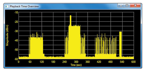
Figure 5 Visual inspection of the captured spectrum data revealed four regions of interest.
Extracting Information from Interference
The signal-analysis software was used to visually inspect the captured data for signs of suspicious interferers. An overview measurement of magnitude versus time for the full 600-second capture revealed four distinct periods of potentially interesting activity (see Figure 5). In the region between approximately 230 and 350 seconds, a large spike appeared around the 270 second mark. Focusing on this area provided informative views in the spectrogram and persistence spectrum formats, as shown in Figure 6. In the spectrogram display (top), two bursts of the interferer intrude into the spectrum of an orderly carrier signal.
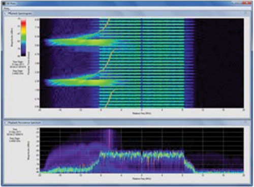
Figure 6 Spectrogram display shows two bursts of the interferer.
The “standard search” capability in the software was used to identify the orderly carrier, which was believed to be an 802.11g signal. As shown in Figure 7, the search parameters include a confidence limit (set to 40 percent in this case), a candidate type of standard (here set to 802.11a/g) and the time range of interest within the captured data (set to 250 to 300 seconds). The confidence limit helps reveal signals that look similar to an ideal wireless standard. This value defines the desired level of correlation between the reference and a captured signal. Using a value of less than 100 percent provides clues into how severely the interference is affecting the victim signal.
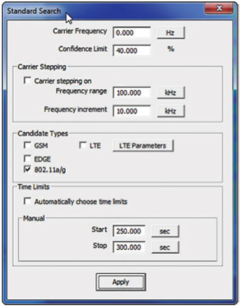
Figure 7 "Standard search" dialogue box used to select parameters.
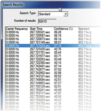
Figure 8 The search results summary reveals areas of high and low confidence.
In this case, the search found more than 92,000 instances of signals that resembled the 802.11g reference. As expected, there were regions of severe degradation that occurred when the interference signal appeared: as shown in Figure 8, correlation dropped from 80-plus percent to less than 50 percent. For each region of poor correlation, the results were examined using a spectrogram display (Figure 9). This 60 µs (top to bottom) spectrogram display shows the interferer disrupting the reference sequence (3 to 11 µs) and payload (11 µs and above) of the 802.11g signal. This pinpointed the five-second span during which the interferer was operating.
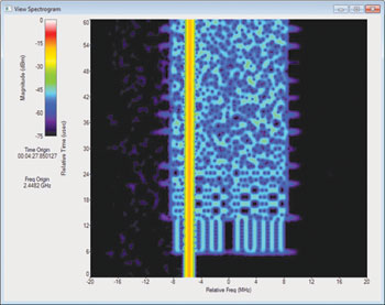
Figure 9 Spectrogram display showing the interferer.
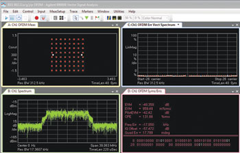
Figure 10 Key indicator of modulation quality when interferer is dormant.
The associated I/Q data was then exported to the VSA software for detailed analysis. In the time prior to the interference, the key indicators of modulation quality were all good, as shown in Figure 10. The OFDM constellation (upper left), EVM (upper right) and spectrum (lower left) are normal. When the interference was active, the impact was catastrophic: the pilots and payload carriers were completely disrupted as the interfering signal walked through the transmission (see Figure 11). The OFDM constellation (upper left) is shattered, EVM (upper right) is erratic and a large spike is present in the frequency spectrum (lower left).
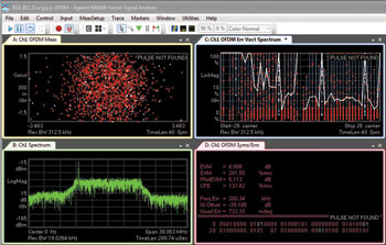
Figure 11 Key indicator of modulation quality with interferer present.
Revealing the Scenario
This incident occurred in an Internet café. The unintentional jammer was a microwave oven and it disrupted the Wi-Fi connectivity every time the staff warmed a pastry or sandwich. Even though this was a relatively benign situation, the suggested procedure works equally well in scenarios that involve interference that affects radio communications, telemetry links, flight range operations, signal intelligence
(SIGINT), system interoperability, and so on. It also supports the three most common usage scenarios: record in theater and playback in the lab, record in the lab and playback in the lab, and create in the lab and playback on the range.
Deploying Effective Tools
Various types of interference can impact critical defense systems. When that interference is an intentional threat, it is important for designers and researchers to have effective “RF forensic tools” — such as those shown here — that can unravel what actually happened in the electromagnetic spectrum. Extracting useful RF information is the first step in developing effective mitigation strategies and solutions.