
Two decades ago, oscillators were typically designed by starting with a topology named for its discoverer, such as Colpitts or Pierce, and then analytically or empirically modifying element values to achieve a desired result. Later, the application of linear CAE tools provided more options and opportunity. The use of nonlinear analysis, along with other recent advancements, has contributed to the maturity of the knowledge. However, misunderstanding still abounds. This article briefly reviews classic linear analysis techniques, extends this analysis to closed-loop concepts, reviews a recent contribution by Randall and Hock, and adds nonlinear analysis to develop a thorough but intuitive feel for the oscillation phenomena. Finally, the nature of oscillator startup is illustrated using a new oscillator topology.
| |||||||||

A perfectly matched non-inverting amplifier with adjustable gain, cascaded with a series L-C 100 MHz resonator with infinite capacitor Q and an inductor Q of 38, is shown in Figure 1. This cascade is driven by a 50![]() source into a 50
source into a 50![]() load. The transmission amplitude responses with amplifier gain of 6, 3 and 0 dB are given in green, blue and red, respectively. The transmission phase is given in cyan. The finite inductor Q introduces an insertion loss in the resonator given by
load. The transmission amplitude responses with amplifier gain of 6, 3 and 0 dB are given in green, blue and red, respectively. The transmission phase is given in cyan. The finite inductor Q introduces an insertion loss in the resonator given by

The reactance of the 2533 nH inductor at 100 MHz is 1591.53![]() . With 50
. With 50![]() terminations at each end of the resonator, the total load resistance is 100
terminations at each end of the resonator, the total load resistance is 100![]() and the loaded Q is 15.91. Since the capacitor Q is infinite, the unloaded Q equals the inductor Q of 38.4. The resulting resonator insertion loss is 3 dB. Therefore, with 6 dB of amplifier gain, the cascade gain is 3 dB. An oscillator is formed by connecting port 2 to port 1, thus closing the loop. The signal level builds at the frequency where the transmission phase is zero degrees. In this simplified example, the phase crosses zero degrees exactly at the resonant frequency of the resonator. The steepness of this transmission phase slope establishes the phase noise and long-term stability of the oscillator. The effects of amplifier transmission phase shift, the cascade input and output match, and nonlinear behavior are discussed later.
and the loaded Q is 15.91. Since the capacitor Q is infinite, the unloaded Q equals the inductor Q of 38.4. The resulting resonator insertion loss is 3 dB. Therefore, with 6 dB of amplifier gain, the cascade gain is 3 dB. An oscillator is formed by connecting port 2 to port 1, thus closing the loop. The signal level builds at the frequency where the transmission phase is zero degrees. In this simplified example, the phase crosses zero degrees exactly at the resonant frequency of the resonator. The steepness of this transmission phase slope establishes the phase noise and long-term stability of the oscillator. The effects of amplifier transmission phase shift, the cascade input and output match, and nonlinear behavior are discussed later.
The loaded Q of the oscillator is proportional to the steepness of the transmission phase slope

where ![]() and
and ![]() are in radians. Because the group delay, td, is equal to minus the rate of change of radian phase with respect to radian frequency, the form
are in radians. Because the group delay, td, is equal to minus the rate of change of radian phase with respect to radian frequency, the form

is convenient because network analyzers measure group delay. While the open-loop may be analyzed at any impedance which best matches the cascade, 50![]() is convenient because the prototype cascade may be measured with a network analyzer.
is convenient because the prototype cascade may be measured with a network analyzer.
| |||||||||

In Figure 2, the cascade open loop is closed using a mathematical dual backward-wave coupler with no insertion loss and 0 dB coupling value. A signal that travels to the right is injected at port 1 and is extracted at port 2. Notice that with the loop closed the gain is approximately 7.6 dB (as shown in red) even though the open-loop gain is –3 dB. When the net open-loop gain is 0 dB the closed-loop gain approaches infinity.
The realization that the closed-loop gain is infinite and the presence of noise in the amplifier have encouraged recent theories to suggest that the oscillator output is nothing more than a limited bandwidth noise source. This viewpoint is helpful in that it provides another perspective on oscillator phenomena. However, it is important to keep in mind that an oscillator theory is possible without the existence of noise. It will be shown that the noise viewpoint can be misleading when oscillator starting is considered later in the article.
In Figure 3, the loop is closed and the reflection coefficient is measured at the input of the amplifier. The red trace corresponds to a 0 dB amplifier gain and a net open-loop gain of –3 dB. The reflection coefficient is less than 1, inside the circumference of a unity radius Smith chart, representing a positive real component of the impedance. The blue trace corresponds to a net loop gain of zero dB and the green trace a net loop gain of 3 dB. In the later case, the reflection coefficient is greater than one representing a negative component of the impedance. If the reflection coefficient is greater than one, the system will oscillate at the frequency where the reflection coefficient passes through the real axis on a Smith chart. In recent years, much has been written that these conditions are not sufficient and that the Nyquist criteria must be used. When it is realized that the real axis represents either a 0° or 180° reflection coefficient, this confusion is avoided. Furthermore, the magnitude of the reflection coefficient is a function of the selected reference impedance and offers little intuitive insight. If the port real and imaginary impedances are plotted rather than the more popular reflection coefficient, these issues are avoided. A word of caution — not all one-port oscillators are of the negative resistance type. Some are negative conductance oscillators. For a complete description of this and other issues covered in this article, please refer to the Oscillator Design Series.1
| |||||||||

The open-loop analysis, the closed-loop analysis and one-port reflection analysis are simply different perspectives of the oscillation phenomena. The remainder of the article deals with the initial design of the oscillator based on the open-loop perspective, which provides insight into multiple oscillation phenomena that should be considered.
The Randall and Hock Technique
The open-loop analysis method terminates the cascade with equal, resistive, source and load impedances. Any resistance that best matches the cascade input and output impedances may be used. If the cascade is designed for approximately 50![]() , the open-loop gain and phase are easily verified using a network analyzer, and so all design aspects including parasitics are considered before an oscillator is formed by closing the loop.
, the open-loop gain and phase are easily verified using a network analyzer, and so all design aspects including parasitics are considered before an oscillator is formed by closing the loop.
However, because the cascade is generally not perfectly matched to the selected reference impedance, an error is introduced into the analysis. A number of techniques have been proposed to overcome this analysis error. An elegant solution was proposed by Randall and Hock.2 They derived an expression for the self-terminated open-loop gain and phase as a function of the normal open-loop scattering parameters. Their expression for the complex gain, G, is
The S-parameters may be measured at any selected reference impedance and the resulting value of G is unchanged. Notice that if S11, S22 and S12 are small, then G = S21.
| |||||||||

When is it necessary to utilize Randall and Hock's expression rather than the uncorrected open-loop gain? Consider the plots on the left side of Figure 4. The input and output return losses of this cascade are 19.9 and 3.7 dB, respectively. The reverse scattering parameter, S12, is –25 dB. While the input return is excellent, the output return loss is poor. Nevertheless, the accuracy of the uncorrected gain and phase, as compared to the corrected gain and phase, is good. The phase slope of the corrected transmission phase shown in cyan is greater, revealing that the oscillator loaded Q is slightly higher than anticipated by the uncorrected open-loop response.
The plots on the right are for an amplifier-resonator cascade with input and output return losses of 2.2 and 1.4 dB, respectively. Even with return losses this poor, the uncorrected gain is in error by only 3 dB and the frequency estimate is only 4 percent too high. If the cascade return losses are controlled to 6 dB or better, the benefits of the corrected gain expression are marginal.
Nonlinear Open-loop Analysis
Once the linear oscillation criteria are established for the open-loop cascade, the loop is closed, and the oscillation level builds until the device nonlinearity absorbs the excess gain margin at the phase-zero crossing frequency. The literature abounds with examples of closed-loop nonlinear analysis using SPICE or harmonic balance-based simulation. However, once oscillation commences, the available data are inadequate to fully reveal the complex nonlinear phenomena that occur. It is helpful to consider nonlinear effects prior to closing the loop. The benefit is the revelation of potential pitfalls.
A 2N2222 transistor amplifier, with a 680![]() shunt feedback resistor and a 4.7
shunt feedback resistor and a 4.7![]() series feedback resistor, is shown in Figure 5. These feedback resistors moderate the gain at low frequency, flatten the frequency response, and result in small-signal input and output return losses of 12.6 and 14.4 dB, respectively, in a 50
series feedback resistor, is shown in Figure 5. These feedback resistors moderate the gain at low frequency, flatten the frequency response, and result in small-signal input and output return losses of 12.6 and 14.4 dB, respectively, in a 50![]() system.
system.
Shown in red in Figure 6 is the gain of this amplifier, not as a function of frequency, but rather at 10 MHz as a function of the input drive level from –20 to 10 dBm. This analysis was performed using the HARBEC harmonic balance simulator.3 A low frequency is used to facilitate measurement of time-domain waveforms with an oscilloscope. At low drive, the gain is approximately 12 dB. As the input level increases, the device becomes increasingly nonlinear and the gain decreases. The gain has compressed 1 dB at –11 dBm input and the gain is 0 dB at 8 dBm. Plotted in green is the output power at the 10 MHz fundamental. The output power at the 1 dB compression is approximately 0 dBm and the saturated output power is 7.5 dBm.
|
|

It is easy to focus on the amplitude characteristics of the cascade. However, it is the phase that determines the oscillation frequency, the phase noise performance and the long-term stability versus temperature, the device and tolerances. The transmission phase of the amplifier as a function of drive level is shown in blue. The phase shift is well behaved, varying less than 1°, up to approximately 4 dBm of drive and 9 dB of gain compression. At higher drive levels the phase shift is more severe. A change in phase as the device becomes nonlinear would result in a shift in frequency. This can indirectly influence the gain margin and the loaded Q of the cascade. It is advisable to evaluate the nonlinear phase characteristics of any amplifier used in an oscillator.
The input return loss of the amplifier versus drive level is shown in Figure 7. As the drive is increased in this amplifier, the input impedance shifts to the left toward an improved match. Achievement of the steady-state oscillation condition is often described as a gain reduction to a net loop gain of 0 dB. In reality, not just compression, but the compression, transmission phase and match, all shift until the net loop gain is 0 dB at the final phase-zero crossing.
This amplifier is well behaved. When this amplifier is cascaded with a resonator with loss, and power is coupled out of the circuit to a load, the net small-signal open-loop gain margin is approximately 2.5 dB, as shown in Figure 8. Up to approximately 9 dB of compression, the phase and impedance shifts are minimal for this amplifier. With only a 2.5 dB of gain compression required, the cascade oscillation frequency and loaded Q will be almost identical to the linear analysis. All amplifiers are not this well behaved.
|
|


Nonlinear Oscillator Analysis
Once the open loop is well understood and characterized, the next step is nonlinear analysis of the oscillation mode. Harmonic balance simulation is applied to the cascade in Figure 9 to determine the nonlinear oscillation frequency, the output level and the harmonic performance. Harmonic balance simulates a steady-state condition so starting must be artificially induced. A schematic of the starting circuit is shown in Figure 10. The three-port block is the open-loop cascade. Ports 1 and 2 are shorted together to close the loop. Power is taken from port 3, which becomes the only port of the closed-loop oscillator.
|
|


The starting circuit consists of a signal generator VS1 and a high Q series L-C network tuned to the fundamental at fo. The frequency and voltage level of the generator are adjusted to be exactly equal to the natural voltage at the shorted ports, thus resulting in no net current flow in the generator. This is accomplished by optimizing until the current in the generator branch is zero. In order that the generator does not short harmonics, the frequency of the high Q series L-C network is kept resonant at fo. At harmonic frequencies, this network presents a high impedance and does not load the oscillator.
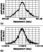
The simulated output spectrum of the oscillator is shown in red. The frequency and level were optimized until the generator current was only 7.8 ![]() A. The oscillation frequency is 9.94 MHz and the output power is –4.5 dBm. The second harmonic is –42 dBm, or 37.5 dB below the carrier. This excellent harmonic performance is achieved by extracting output power from the resonator, which serves as a signal filter. Load frequency pulling is reduced by decoupling the load with a low reactance capacitor in parallel with the load. Superimposed on the simulated output spectrum, the measured data taken with an Avantest R3265A spectrum analyzer is shown in green.
A. The oscillation frequency is 9.94 MHz and the output power is –4.5 dBm. The second harmonic is –42 dBm, or 37.5 dB below the carrier. This excellent harmonic performance is achieved by extracting output power from the resonator, which serves as a signal filter. Load frequency pulling is reduced by decoupling the load with a low reactance capacitor in parallel with the load. Superimposed on the simulated output spectrum, the measured data taken with an Avantest R3265A spectrum analyzer is shown in green.
Loaded Q: A Silver Bullet
In 1966, Leeson published a formula for the single-sideband (SSB) phase noise of a feedback oscillator that is still widely used.4 His formula shows that the loaded Q is the most effective design parameter for improving oscillator phase noise. In fact, the phase noise improves with the square of the loaded Q. It is critical to grasp the distinction between loaded Q and unloaded Q.1
It is less well published that an increase in loaded Q improves other oscillator performance specifications as well. Recall that it is the transmission phase zero that establishes the oscillation frequency. The loaded Q is proportional to the steepness of that transmission phase. It is also critical to realize this is not referring to the phase slope of the reflection coefficient of an oscillator analyzed by the one-port method. From Equation 2 the frequency shift is given by
and after conversion from radians to degrees

For example, the shift of the transmission phase of the discrete 10 MHz amplifier caused by 3 dB of compression is approximately 0.25°. The loaded Q at the phase-zero crossing is 5.6. Notice that the loaded Q at the oscillation frequency is approximately half of the loaded Q at the maximum phase slope. This is because the phase shift of the amplifier and resonator are not proper to align the phase-zero crossing at the maximum phase slope. An optimum oscillator design would correct this issue. This could be accomplished by using an inductive choke rather than the resistor R4. A resistor was used here for simplicity.
From Equation 6, for this case with 0.25° of compression phase shift and a loaded Q of 5.6, as the amplifier compresses 3 dB, the frequency shift is only 3.9 kHz, or 0.039 percent. This is a mere fraction of the frequency error that is introduced by component tolerance and therefore raises the confidence in linear open-loop analysis of well-designed oscillators.
Notice, from Equation 6, that the frequency shift introduced by a phase perturbation is inversely proportional to the loaded Q. Factors that influence the frequency of an oscillator do so by perturbing the transmission phase. Therefore, increasing the loaded Q not only improves Leeson's phase noise, but it reduces long-term instability and phase noise introduced by the following factors:
- Temperature changes in both active and passive components
- Bias changes introduced by power supply drift and noise
- Nonlinear effects in the active device
- Load-pulling introduced by variation in the load impedance
- The loaded Q is absolutely critical to oscillator performance.
Oscillator Starting
| |||||||||

Perhaps no misconception is as entrenched in oscillator lore as the cause of starting. Ask an engineer what causes the oscillator to start and the response is noise; noise within the resonator bandwidth builds until a steady state operating level is achieved. The noise theory is so compelling that engineers may believe that oscillator phase is undefined and uncontrollable.
The open-loop cascade of a 10 MHz oscillator was designed without bypass capacitors or choke inductors in the bias circuitry. The capacitor C1 is required for nonlinear open-loop analysis so that the source does not shunt the base bias circuitry. In the final oscillator, the resonator capacitor C3 provides that function and C1 is not required. So, the only reactances are within the resonator.
A photograph of the prototype oscillator is shown in Figure 11. An unusual feature of this test oscillator is that the power supply is a low frequency square-wave. The measured starting waveforms with applied square-wave peak voltages of 1.85, 2.9 and 4 V are given in Figure 12. These waveforms were captured with an Agilent 54855A oscilloscope using the TESTLINK module of GENESYS.
| |||||||||

With a supply of 1.85 V, the transistor collector current is only 100 ![]() A and the simulated open-loop gain is approximately –25 dB, far below unity gain. The sudden application of a voltage on the resonator results in an output waveform ringing that dies with time because of inadequate cascade gain margin. With a peak square-wave voltage of 2.9 V, the gain margin is unity and the output level remains relatively constant. This is not a practical operating point because there is no margin for temperature or device tolerances. Finally, with an applied square-wave peak voltage of 4.0 V, the simulated small-signal open-loop gain is approximately 2.5 dB and the signal level builds until nonlinear action establishes the steady-state operating point.
A and the simulated open-loop gain is approximately –25 dB, far below unity gain. The sudden application of a voltage on the resonator results in an output waveform ringing that dies with time because of inadequate cascade gain margin. With a peak square-wave voltage of 2.9 V, the gain margin is unity and the output level remains relatively constant. This is not a practical operating point because there is no margin for temperature or device tolerances. Finally, with an applied square-wave peak voltage of 4.0 V, the simulated small-signal open-loop gain is approximately 2.5 dB and the signal level builds until nonlinear action establishes the steady-state operating point.
The starting waveforms depicted here were captured with 500 ms of persistence with an applied square-wave period of 5 ![]() s. The figure therefore represents approximately 100,000 repeated and superimposed starting waveforms triggered off the leading edge of the square-wave supply voltage. There is little observable jitter in the starting waveform. The oscillator starts instantly at the same phase on each start. This is not a process dictated entirely by noise. This waveform appears to be a gated oscillator, but it is not. These are multiple oscillator starting waveforms.
s. The figure therefore represents approximately 100,000 repeated and superimposed starting waveforms triggered off the leading edge of the square-wave supply voltage. There is little observable jitter in the starting waveform. The oscillator starts instantly at the same phase on each start. This is not a process dictated entirely by noise. This waveform appears to be a gated oscillator, but it is not. These are multiple oscillator starting waveforms.
What is happening? Because the amplifier has no bypass capacitors to charge, the amplifier becomes active as soon as power is applied. The application of the supply voltage begins charging the resonator capacitor C2 through the small resistor R4, and to a lesser extent, C3 through R4 and R2. The fast charging rate of R1 and C2 causes the resonator to ring at its natural frequency. It is this ringing voltage that starts the oscillator with a controlled phase.
The initial amplitude of this ringing waveform is approximately 50 mV peak as observed in the starting waveform with 0 dB net loop gain. With a loaded Q of 5.6 and an amplifier with a 3 dB noise figure, and 1.78 MHz of 3 dB bandwidth (9.95 MHz/5.6), even if the noise is correlated over this bandwidth, the open-loop peak noise voltage is 1.2 ![]() V, forty times lower than the initial ringing signal.
V, forty times lower than the initial ringing signal.
This experiment was designed so that the amplifier is active immediately with the application of the supply. As a result, the oscillator starts instantly, with controlled phase and unobserved jitter. While formulas have been derived and published to predict the oscillator starting time based on noise analysis and loaded Q, in practice, starting is often determined by the time constants in the amplifier bias network, the rise time of the supply voltage, and the charging and ringing characteristics of the resonator. The typical oscillator starts because it is turned on. An exception is an oscillator that uses a well-balanced differential amplifier that does not ring the resonator, as might exist with an IC-based oscillator.
References
- R. Rhea, "Oscillator Design," Desktop Tutorial CD Series, Noble Publishing, Atlanta, GA, www.noblepub.com.
- M. Randall and T. Hock, "General Oscillator Characterization Using Linear Open-loop S-Parameters," IEEE Transactions on Microwave Theory and Techniques, Vol. 49, No. 6, June 2001, pp. 1094–1100.
- Users Guide, GENESYS V2003.3, Eagleware Corp., Norcross, GA, pp. 125-142, www.eagleware.com.
- D.B. Leeson, "A Simple Model of Feedback Oscillator Noise Spectrum," Proceedings of the IEEE, February 1966, pp. 329–330.
Randy Rhea is a graduate of the University of Illinois (1969) and Arizona State University (1973). He worked briefly at Boeing Co. and Goodyear Aerospace, and for 14 years at Scientific-Atlanta, where he became principal engineer. He founded Eagleware Corp. in 1985 and Noble Publishing in 1994. He has authored numerous technical papers, the books Oscillator Design and Computer Simulation and HF Filter Design and Computer Simulation, and numerous RF/microwave tutorial CDs.
Bill Clausen holds BSEE and MSEE degrees from the University of South Florida and is a member of Tau Beta Pi and MTT IEEE. He is currently product manager at Eagleware Corp., where he is responsible for the continuous development of the company's product line, as well as application and support. Before joining Eagleware, he was an RF and microwave/ optics applications engineer with HP/Agilent for 23 years. Prior to his career with HP/Agilent, he held staff engineer positions at Trak Microwave and Sperry Microwave.