
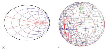
Fig. 1 Representation of the 2D (a) and 3D (b) Smith charts.3
The mathematical theory of the 3D Smith chart1 unifies active and passive microwave circuit design on the surface of a Riemann sphere. The reflection coefficient plane is mapped stereographically through the South Pole on the surface of a unit sphere. As a result, the classical 2D Smith chart including the passive loads2 is mapped stereographically into the North hemisphere, while the circuits with negative resistance (that are outside the classical planar Smith chart) are mapped into the South one. The East hemisphere is the place of inductive circuits, whereas the West hemisphere hosts the capacitive circuits. Meantime, the Greenwich meridian is the locus of pure resistive circuits (see Figure 1, where the constant resistance r and reactance x circles are drawn in blue and red, respectively).
The 3D Smith chart differs from previous attempts4 to generalize the planar 2D Smith chart in a fundamental way: the way in which infinity is treated. The preceding theories fail to merge the active and passive worlds in a simple and rigorous manner, since they propose an empirical solution to map an infinite region into a finite surface. These approaches turned into complicated transforming equations, making the visual and intuitive interpretation of microwave problems very difficult.
In this article, how the 2D and 3D Smith charts deal with the infinite regions are first described. Next, the advantages of using the 3D Smith chart to represent both active and passive loads are illustrated with two examples: the stability circles of an amplifier and the impedance of a microwave oscillator.
Treatment of Infinity in Smith Charts
The infinite region of the normalized impedance or z-plane is due to the open circuit, because the magnitude of the input impedance grows to infinity as the load tends to an open circuit. Since in practical applications, impedances can be found close to the open circuit, it is rather uncommon to use the z-plane to perform a visual representation of loads.
For the reflection coefficient plane (ρ-plane), the infinite region corresponds to the load with the same magnitude and opposite sign to the characteristic impedance of the line (that is the infinite mismatch or z = –1 in normalized impedance terms). Although it denotes a particular active load, this input impedance is important in some practical applications such as oscillator design. To be able to represent the infinite mismatch, practitioners can use a planar Smith chart plotted in the 1/ρ-plane called negative Smith chart.5 This graphical representation gives an important role to the infinite mismatch, which is placed in its center, but moves the matched load (ρ= 0) to infinity. Analogously, the open circuit is placed in the center of the normalized admittance or y-plane, where another important load, the short circuit, is thrown to infinity.
It can be concluded that all the usual 2D planar representations are unable to keep these four key impedances (open circuit, short circuit, matched load and infinite mismatch) in a bounded region. In fact, all these planes extend to infinity, where one of the aforementioned key loads is located.
Maxime Bocher, born in 1867 in Boston, professor at Harvard University and president of the American Mathematical Society (1908-1910), was the one that finalized the theory of inversive geometry. The Bocher Memorial Prize is awarded for outstanding achievements in Mathematics appearing in an American journal,6 and was awarded in 1933 to Norbert Wiener, who played a major role in Information Theory.
Bocher established the theory of the direct inversive and indirect inversive transformations,7 respectively,
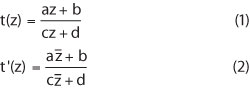
where a, b, c and d are arbitrary complex numbers satisfying ad – bc =/ 0 and z is the extended complex conjugate of the complex variable z. These two transformations map generalized circles (that is circles and infinite lines) into generalized circles, keep the magnitude of the angles and maintain or reverse their orientation. There was a problem with these transformations concerning the points that were thrown at infinity. In his article,8 Bocher maintained his well-known attitude of seeking for the simplest solution to solve and clarify each problem and argued that points thrown to infinity by inversive transformations should form a single point on the Riemann sphere. In fact, he showed that Equations 1 and 2 were always mapping lines and circles into circles on the Riemann sphere and forming a group under the composition of functions.
He proposed a practical conception of infinite regions and his theory of inversive geometry was used by famous mathematicians such as Klein, Caratheodory and Mandelbrot, and in the arts by Escher.
The 2D Smith chart is a graphic representation of the r-plane, including the constant resistance and reactance lines in the z-plane transformed by means of the Möbius transformation
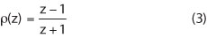
Since Equation 3 is an inversive transformation, it maps infinite lines in the z-plane in generalized circles in the ρ-plane. All the lines in the z-plane extend to infinity and, therefore, all its transformed circles pass through ρ= 1 (the reflection coefficient of the open-circuit). An infinite region of the z-plane is compressed around this point (that is an accumulation point), as also reveals the singular behavior of the transformation between the ρ-plane and the z-plane (that is the reciprocal transformation to Equation 3) in this particular point. On the other hand, the region around the short circuit (ρ= 1) is expanded by the Möbius transformation.
The 2D Smith chart successfully compiles in a bounded region the unit circle and all of the passive loads with the matched load in its center. Although the passive loads are the more common ones, certain applications involve the use of active devices, whose impedances can be very far from the unit circle (for instance in oscillators or negative resistance amplifiers, to cite a few). Moreover, in other applications, it can be interesting to represent both active and passive loads simultaneously (for example, stability circles in amplifiers, representation of the impedance of devices whose input resistance can be positive or negative depending on the bias point or frequency, or mixed problems involving both active and passive devices). The 2D Smith chart has limitations in these applications, mainly because the Möbius transformation expands the region occupied by the active loads to infinity.
These limitations are successfully addressed by the 3D Smith chart. To build this graphical representation, one must first place the ρ-plane in the equatorial plane and next perform its stereographical projection from the South Pole in a Riemann sphere of unit radius.1 Proceeding in this way, the passive loads will be placed in the North hemisphere of the sphere and the active loads are located in the South hemisphere, packaging all loads in a bounded sphere of unit radius without resorting to infinity. Moreover, the four key loads occupy especially important points of the sphere: the matched and infinite mismatch loads are placed in the North and South Pole, respectively, whereas the West Pole contains the open circuit and the East Pole is the short circuit (the West and East Pole are the poles of the sphere with respect to the Greenwich meridian plane, or in other words, the points of the sphere with maximum and minimum x-coordinate, respectively).
It can also be proven that the same representation can be obtained, if the impedance plane is placed in the Greenwich meridian plane and the stereographic projection to the unit sphere is performed from the West Pole. This property proves the completeness of the 3D Smith chart, since both the r-plane and the z-plane will be obtained after performing the inverse stereographic projection in the two main planes cutting the Riemann sphere.
The 3D Smith chart has a wide number of properties that can be helpful to solve microwave problems graphically.1 In fact, it has more properties than the planar Smith chart due to its completeness. The stereographic projection is also a conformal mapping, thus transforming circles in the 2D Smith chart into circles in the surface of the 3D Smith chart. In addition, infinite lines in the planar Smith chart are mapped into circles in the Riemann sphere passing through the South Pole (the locus of the infinite mismatch load), whereas finite lines are transformed into circle arc sections. The same can be stated for circles and lines drawn in the impedance and admittance planes. As a result, and similarly to the 2D Smith chart, a wide variety of microwave problems can be solved graphically in this new tool by drawing and intersecting circles.
Application Examples
In order to work with negative impedances, engineers have to either use different tricks or face scaling problems, which causes problems with the task of handling both active and passive microwave on the same chart. These problems disappear on the 3D Smith chart, where infinity becomes a handy issue.
Amplifier Stability Circles
One of the applications that reveal the limitations of the planar Smith chart and the advantages of the 3D Smith chart is the stability analysis of microwave amplifiers. To guarantee the stability of the amplifier and prevent unexpected oscillations, this analysis must be performed over a very wide frequency range. At each frequency, a stability factor is first computed to determine whether the amplifier is conditionally or unconditionally stable.9,10 If the amplifier is conditionally stable, it is required to plot both the source and load instability regions, which define the loads at the input and the output of the amplifier that should be avoided to prevent a potential oscillation at this particular frequency.
In the ρ-plane, and therefore in the 2D Smith chart, the boundary between stability and instability regions are circles. The center and radius of the source and load stability circles can be easily computed from the S-parameters of the transistor (or, in general, the active circuit providing the amplification).9,10 In most cases, however, one or both circles include active loads, thus being placed partially outside of the 2D Smith chart. In a wide frequency range, this problem generates visualization problems in 2D, due to the scaling required to be able to plot the entire stability circles, identify the problematic regions and look for a possible solution.
The 3D Smith chart does not require any type of scaling, since all the active and passive loads are successfully represented in a bounded surface. Moreover, and due to properties of the stereographic projection, the stability circles in the planar Smith chart transform into circles in the Riemann sphere.
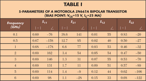
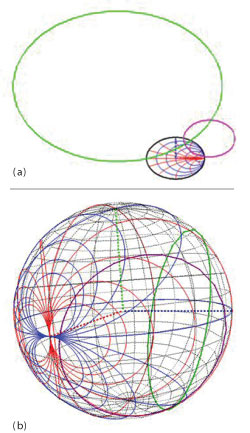
Fig. 2 Representation in the 2D (a) and 3D (b) Smith charts of the stability circles of a Motorola 2N667A bipolar transistor at 100 MHz.
To illustrate these concepts, the stability of a Motorola transistor, with S-parameters given in Table 1, has been analyzed at 100 MHz. Figure 2 depicts the source (in green) and load (in magenta) stability circles of this conditionally stable transistor in both the 2D and 3D Smith charts. To visualize the complete circles, the ρ-plane must be scaled in the 2D representation. This scaling reduces the 2D Smith chart, thus making it more difficult to get a visual insight of the problem even for a single frequency.
The instability regions in the 3D Smith chart correspond to the loads in the surface of the sphere delimited by the stability circles and not containing the North Pole. It can be easily seen that the output instability is due to sources with low and moderate impedance magnitude, and inductive or slightly capacitive character. The input or load instability, on the other hand, can be caused by inductive passive loads with a high quality factor Q. Using this information, the engineer can add elements into the amplifier circuit to move the source and load instability circles to the South hemisphere.
Oscillator Design
To obtain an oscillator at a specified frequency, the microwave active circuit must be designed to provide an infinite reflection coefficient at such a frequency. This requires moving to infinity in the reflection plane, thus being useless in a planar Smith chart representation. To solve this type of problem graphically, two solutions are normally considered: (i) using a 1/ρ-plane or negative Smith chart representation5 or (ii) plot the conjugate impedance of some circuits10 in the 2D Smith chart. Both solutions require combining two different types of planar representations to plot the loads.
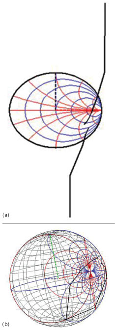
Fig. 3 Input impedance (in black) of a microwave oscillator at 1 GHz in both the 2D (a) and 3D (b) Smith charts.
Figure 3 shows the 2D and 3D Smith chart representation of the input impedance (in black) of a microwave oscillator at 1 GHz based on an Infineon BFP 640 bipolar transistor designed in the literature.10 The 2D Smith chart is incapable of plotting the impedance of the oscillator close to the resonant frequency, whereas it can be successfully plotted in the 3D Smith chart without using a different type of representation. These examples show the practical use of the 3D Smith chart.
References
- A.A. Müller, P. Soto, D. Dascalu, D. Neculoiu and V.E. Boria, “A 3D Smith Chart Based on the Riemann Sphere for Active and Passive Microwave Circuits,” IEEE Microwave and Wireless Components Letters, Vol. 21, No. 6, June 2011, pp. 286-288.
- P. H. Smith, “Transmission-line Calculator,” Electronics, Vol. 12, No. 1, January 1939, pp. 29-31.
- 3D Smith Chart Application available at www.3dsmithchart.com/, last accessed in November 2011.
- Y. Wu, Y. Zhang, Y. Liu and H. Huang, “Theory of the Spherical Smith Chart,” Microwave and Optical Technology Letters, Vol. 51, No. 1, January 2009, pp. 95-97.
- H.F. Lenzing and C. D’Elio, “Transmission Line Parameters with Negative Conductance Loads and the “Negative” Smith Chart,” Proceedings of the IEEE, Vol. 51, No. 3, March 1963, pp. 481-482.
- W.F. Osgood, "Maxime Bocher- A Biographical Memoir,” National Academy Press, Biographical Memoirs, Vol. 82, WA, 2002.
- D.A. Brannan, M.F. Esplen and J.J. Gray, “Geometry,” Cambridge University Press Cambridge, UK, 2007.
- M. Bocher, “Infinite Regions of Various Geometries,” Bulletin of the American Mathematical Society, Vol. 20, No. 4, 1913, pp. 185-200.
- J.F. White, “High Frequency Techniques: An Introduction to RF and Microwave Engineering,” John Wiley & Sons, Hoboken, NJ, 2004.
- R. Gilmore and L. Besser, “Practical RF Circuit Design For Modern Wireless Systems, Vol. II: Active Circuits and Systems,” Artech House, Norwood, MA, 2003.
Andrei Müller obtained an MSC in Telecommunications Engineering in 2005, a second MSC in Microsystems in 2007 and a PhD degree in Telecom Engineering from UPB-Bucharest in 2011. He performed microwave related research stages at HFT-Munich-Germany (2007-2008) and at CEFIM-Pretoria-South Africa (2009). During his PHD, Andrei chose to use a fellowship in order to complete a seven month stage in pure mathematics at IUMPA, Valencia, Spain, 2010. His current interests are the extensions of the 3D Smith chart tool (www.3dsmithchart.com) and applications of projective, inversive and non-euclidian geometry in EM design.
Dan C. Dascalu is the founder and the first Director General of IMT (1993-2011), today the National Institute for R&D in Microtechnologies (IMT-Bucharest). He graduated from the Electronics Department of the University “Politechnica” of Bucharest, Romania (1965) and obtained his Ph.D. from the same university (1971). His particular interest was related to transit-time effects. He is a full Member of the Romanian Academy (of Sciences). Prof. Dascalu is now the Coordinator of Center for Nanotechnologies from IMT and President of the Coordinating board of IMT centre for Micro- and NANOFABrication (IMT-MINAFAB). IMT is a hub of micro- and nanotechnologies in Romania (scientific networking, innovation, education) and hosts a European Centre of excellence in RF MEMS and MOEMS.
Pablo Soto received his M.S. degree in Telecommunication Engineering from the Universidad Politécnica de Valencia in 1999, where he is currently working toward the Ph.D. degree. In 2000 he joined the Departamento de Comunicaciones, Universidad Politécnica de Valencia, where he has been a Lecturer since 2002. In 2000, he was a fellow with the European Space Research and Technology Centre (ESTEC-ESA), Noordwijk, the Netherlands. His research interests include numerical methods for the analysis, synthesis, and automated design of passive waveguide components.
Vicente E. Boria received his M.S degree (with first-class honors) and his Ph.D. degree in Telecommunications Engineering from the Universidad Politécnica de Valencia, Spain, in 1993 and 1997, respectively. In 1993, he joined the Departamento de Comunicaciones, Universidad Politécnica de Valencia, where he has been full Professor since 2003. In 1995-1996, he held a Spanish Trainee position with the European Space Research and Technology Centre (ESTEC-ESA), Noordwijk, The Netherlands, where he was involved in the area of EM analysis and design of passive waveguide devices. His current research interests include numerical methods for the analysis of waveguide and scattering structures, automated design of waveguide components, radiating systems, measurement techniques, and power effects (multipactor and corona) in waveguide systems.