
When EM engineers use design and modeling packages they want ease of use, reliability and, most importantly, the ability to design new products that meet the desired purpose quickly and effectively. These were the main considerations when Flomerics developed MicroStripes 7, together with the aim of ‘bringing electromagnetic simulation to every engineer’s desktop.’ This aim appears to have been achieved, as the new features of the simulation software have seen productivity gains of up to 60 percent being reported in recent trials by some design engineers.

One aspect of MicroStripes 7 that sets it apart from other commercial electromagnetic simulation software is the core solver technology, which uses a mathematical technique known as the transmission line matrix method (TLM) to solve the time-honored Maxwell’s equations. The key advantage of TLM is that it is highly efficient in terms of the amount of computer memory and CPU time required per computational cell, meaning that very large problems can be handled.
Significant new enhancements to Version 7 include ‘auto-lumping’ of computational cells, an improved user interface, arbitrary plane wave excitation and parametric sweeps to allow optimum designs to be achieved more efficiently. The company has also recently announced an alliance with Applied Wave Research Inc. (AWR) in which the MicroStripes software will provide full 3D analysis capabilities to users of AWR’s Microwave Office software.
The development of Version 7 recognizes that the current need for 3D EM simulation is expanding rapidly. Engineers are faced with reduced design cycles, increasing frequencies, demanding performance metrics and, of course, cost considerations. Therefore, they need a tool, which is flexible, easy to use, interoperable with CAD, offers intelligent mesh generation, provides a seamless link with current design tools and is cost effective.

In response to these demands the virtual prototyping environment within the new software allows detailed insight into whether the device or component will meet design criteria even before manufacture. This dramatically reduces design iterations and reduction in design costs, making it a tool that truly addresses the challenges faced by the modern RF/microwave engineer.
Auto-lumping
Engineers face an ever-increasing need to solve larger and larger computational problems, which leads to long simulation times and increased computer memory requirements. This is especially so for installed antenna performance, wherein the user models the fine geometric features of a typically small antenna structure in a large and geometrically complex computational volume.

To address this, ‘octree’ meshing is utilized, which progressively and automatically lumps together computational cells in regions remote from the geometric detail. The ultimate size of the lumped cells is limited only by the local permittivity, permeability and highest frequency of interest. This enables critical but electrically small detail to be captured with an exceedingly high resolution mesh, without having a significant impact on the global cell count.
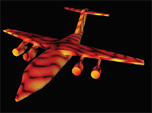
To illustrate the benefit of this feature consider an aircraft measuring 26 m by 26 m by 8 m, which has been imported as a hollow metal object into Version 7. The aircraft is surrounded with free space of 10 m in each direction, giving a total computation volume of about 59,248 m3. The aircraft is illuminated by an off-axis plane wave with maximum frequency of 100 MHz. Figure 1 shows the surface current distribution graph.
What is noticeable is that a very fine mesh is applied to capture the detail of the structure. However, due to the automatic lumping, the total cell count is only about 3.6 million, which is a 99.3 percent savings compared to the graded mesh of 529 million cells before lumping. The lumping is mainly performed inside the aircraft and in the free space, while keeping a fine mesh on the metal surface of the aircraft. Significantly, the simulation was completed within 17 hours on a dual 1.99 GHz AMD Opteron and the memory usage was only 609 Mbytes.
Parametric Sweep
In RF design work, engineers often need to modify features of a design to tune for the best performance. MicroStripes 7 facilitates such tuning by allowing variables and mathematical operators in geometric parameters. The simulation can then sweep a variable in regular steps, between the minimum and maximum set values defined.
As an example of this feature, the horn antenna shown in Figure 2 has variables defining the dimension of the objects in the model. Flare_y is the horn opening in the direction of the Y-axis, which has been given a set of values, swept from 25 mm to 75 mm in two steps. Version 7 automatically applies the variable sweep as part of the simulation. The results for different variable values can then be compared in a single graph. Figure 3 shows the change in the directivity due to different values of flare_y. The red, black and purple traces represent the antenna directivity when flare_y is equal to 25, 50 and 75 mm, respectively.
Radar Cross-section Plane Waves
The extension of the plane wave excitation to allow arbitrary angles of incidence means the mono-static and bi-static radar cross-section (RCS) can quickly and easily be determined. Plane wave incidence from any angle is allowed, with any transverse polarization. RCS results can then be visualized in a 3D far-field plot and in 2D far-field cut planes.

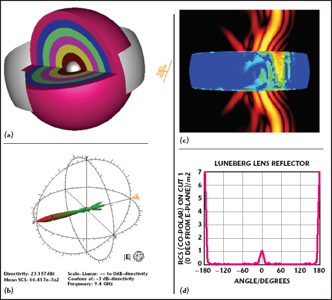
As an illustration, consider the Luneburg lens radar-reflector, shown in Figure 4, which is commonly carried by yachts in order to increase their visibility to larger vessels. This dielectric device is spherical and has a permittivity that varies along the radius. Plane waves incident from any direction are focused to a point on the far surface. To make a retro-reflector, the lens surface in the region of the focus is metalized. Radiation reflected at the focus is collimated in passing back through the lens, and sent back to its original source. In order to show the metal band, the outmost layer of dielectric is hidden. The figure also shows the scattered field for the lens reflector illuminated by a 45° polarized signal. A little yellow Yagi antenna is used to symbolize the propagation direction and polarization of the incident plane wave.
The 3D far-field plot generated by EM simulation software shows a value for the mean scattering cross-section (SCS). If the mouse is moved over the plot, then the varying value for the RCS is reported in the window footer. This value of RCS relates to direction under the mouse and for the plotted polarization, that is, both the directive gain and polarization loss are factored in. Alternatively, the RCS result can be seen in the cuts plots; for example, a co-polar far-field cut is provided in Figure 4.
Software Partnership
Also significant in the development of Microstripes 7 is the partnership that Flomerics has entered into with AWR in order to provide users with an enhanced data transfer using the AWR EM Socket interface. This will enable Microwave Office users to transfer data to the MicroStripes 3D solver, allowing comprehensive analysis of antennas, filters, couplers, interconnects, planar structures and packaging effects. The open architecture format makes this straightforward, yet yields great benefits in terms of re-using data and speeding up the overall RF design flow. A typical example is illustrated in Figure 5, which shows the current flow distribution on a 3 dB coupler.
Conclusion
MicroStripes 7 represents a significant forward leap in electromagnetic modeling software and reinforces the company’s position as a leading provider of 3D electromagnetic virtual-prototyping software. The most significant improvements are an enhanced user interface; automatic octree meshing; intuitive parametric sweeps; and arbitrary plane wave illumination for radar cross-section applications. The alliance between AWR and Flomerics will also significantly improve the design flow between 2.5D and 3D RF/microwave design.
Flomerics,
Hampton Court, Surrey, UK
+ 44 20 8487 3000,
info@flomerics.co.uk,
www.flomerics.com.